2 Methods and Materials
A diverse set of computational tools and methodologies were employed in this study to analyze and interpret complex biomedical data.
2.1 Data Preprocessing
2.1.1 COVID-19 Cell profilling Data
In this study, the data preprocessing stage consisted of the preparation and normalization of a COVID-19 dataset. This dataset contained phenotype features and metadata extracted from multiple images of Vero-E6 cells (African green monkey) infected with Human coronavirus SARS-CoV-2 and treated with 5300 drugs from the Specs Repurposing Library. Each compound was represented in two plate replicates within the set of 32 plates, each containing 384 wells. Fluorescent images were captured using an Image Xpress Micro XLS (Molecular Devices) microscope with a 20× objective using laser-based autofocus. Five labels were used to stain the cells, characterizing seven cellular components, including DNA, Golgi apparatus, plasma membrane, F-actin, nucleoli and cytoplasmic RNA, the endoplasmic reticulum, and the SARS-CoV-2 spike protein. The image files were then stored in grayscale TIFF format.
The open-source image analysis software CellProfiler version 4.0.6 was utilized to extract a total of 2009 morphological features, including size, shape, pixel intensities, and texture, from these images. The initial dataset cleaning involved the removal of features with constant values or missing data and empty features. Numeric columns in the dataset were subsequently isolated into ‘phenotype features’ and ‘metadata’. These features were then averaged on an image level. Features with extreme and outlier standard deviation values (SD < 0.001 and SD > 10000) were also eliminated.
This dataset represents an extensive collection of phenotype features extracted from images, along with associated metadata. Each row in the dataset corresponds to a single image, with each image associated with a specific site within a well. There are 9 sites (numbered 1-9) within each well, and approximately 350-360 wells within each plate, with a maximum of 384 wells per plate. The dataset encompasses 24 plates.
| ImageID | ~ 2000 phenotype features | PlateID | Well | Site | Plate | Plate_Well | batch_id | pertType | cmpd_conc | Flag | Count_nuclei | Batch nr | Compound ID | selected_mechanism |
|---|---|---|---|---|---|---|---|---|---|---|---|---|---|---|
| P03-L2_B03_1 | ……….. values ………. | P03-L2 | B03 | 1 | 03-L2 | specs935-plate03-L2_B03 | BJ1894547 | trt | 10.0 | 0 | 109.0 | BJ1894547 | CBK042132 | estrogen receptor alpha modulator |
| P03-L2_B03_2 | ……….. values ………. | P03-L2 | B03 | 2 | 03-L2 | specs935-plate03-L2_B03 | BJ1894547 | trt | 10.0 | 0 | 121.0 | BJ1894547 | CBK042132 | estrogen receptor alpha modulator |
. . . |54366 rows, 2140 columns|
During the preparation phase, the first step involved dropping empty features, i.e., columns with no values or with a standard deviation (SD) of 0. The dataset was then segregated into numeric columns, further filtered down to ‘phenotype features’ and ‘metadata’. The ‘phenotype features’ included numeric columns excluding those with certain strings such as ‘Metadata’, ‘Number’, ‘Outlier’, ‘ImageQuality’, ‘cmpd_conc’, ‘Total’, ‘Flag’ and ‘Site’. The difference between the number of numeric columns and the number of phenotype features gives the number of ‘metadata’.
numeric_columns = list()
for a in df.columns:
    if (df.dtypes[a]  'float64') | (df.dtypes[a]  'int64') :
        numeric_columns.append(a)

feature_columns = [fc for fc in numeric_columns if ('Metadata' not in fc) & ('Number' not in fc) &
                   ('Outlier' not in fc)  & ('ImageQuality' not in fc)  & ('cmpd_conc' not in fc)  &
                   ('Total' not in fc) & ('Flag' not in fc)  & ('Site' not in fc) ]
The preparation phase also involved removing any features with missing values and those with an SD less than 0.0001.
2.1.1.1 Normalization
Two methods of normalization were employed in this study: an overall approach and a plate-separated strategy. Both strategies utilized Median and Median Absolute Deviation (MMAD) normalization[35]. The normalization was accomplished using the formula:
\[MMAD = \frac{X - DMSO_{median}}{|X_{dmso} - DMSO_{median}|_{median}}\]
where \(X\) denotes the observed feature value, \(DMSO_{median}\) signifies the median value of DMSO, and \(X_{dmso}\) represents the observed feature value of DMSO. The overall strategy applied this formula to the entire dataset at once, whereas the plate-separated strategy applied it independently to each plate, using the local median values of DMSO for normalization within that plate.
dfDMSO = df[df['batch_id'] == '[dmso]']
dfDMSO_Medians = dfDMSO[phenotype_features].median()
dfDMSO_MADs = (dfDMSO[phenotype_features] - dfDMSO[phenotype_features].median()).abs().median()
df_MMAD = df[phenotype_features].copy()
df_MMAD = (df[phenotype_features] - dfDMSO_Medians[phenotype_features])/dfDMSO_MADs[phenotype_features]
df_MMAD.clip(lower=-10, upper=10,  inplace=True)
In the plate separated approach, the same process was applied. However, it was done first by finding local median values for DMSO in each plate and normalizing the measurements in the same plate based on their respective DMSO medians.
df_MMAD_by_plate = pd.DataFrame()

for plate in plates:
    plate_data = df[df['Plate'] == plate]
    df_DMSO = plate_data[plate_data['batch_id'] == '[dmso]']
    df_DMSO_medians = df_DMSO[phenotype_features].median()
    df_DMSO_MADs = (df_DMSO[phenotype_features] - df_DMSO[phenotype_features].median()).abs().median()
    MMAD = (df[df['Plate'] == plate][phenotype_features] - df_DMSO_medians[phenotype_features])/df_DMSO_MADs[phenotype_features]
    df_MMAD_by_plate = pd.concat([df_MMADs_by_plate, MMAD])

df_MMAD_by_plate
The site-level features were normalized at the plate level using the mean and standard deviation of the DMSO sites in the plate. MMAD normalization was chosen due to its robustness to outliers, implying that it functions well even with data containing extreme values. In contrast, other methods, such as Z-score normalization, could be significantly affected by these outliers. Furthermore, MMAD normalization does not require the data to follow a specific distribution, making it a versatile choice for various datasets. The application of two different strategies, one that treated the dataset as a whole and another that treated each plate independently, was done to account for potential variations within and between different plates.
2.1.1.2 Dimensionality Reduction
In this part, several key steps were undertaken to reduce the dimensionality of the data, select the most informative features, and visualize the structure and variability of the data using Principal Component Analysis (PCA). PCA was applied to the dataset to identify the key direction or “a component” that describes most of the data variability. This process helps to transform the original dataset into an updated one where each data point is represented in terms of this component. The PCA algorithm also provides the loadings, or the contribution of each original feature to each principal component.
from pca import pca
import matplotlib.pyplot as plt

X = covid_df.loc[(covid_df['label'] == 'DMSO') | (covid_df['label'] == 'Uninfected') | (covid_df['label'] == 'Remdesivir')][features].values
row_label = covid_df.loc[(covid_df['label'] == 'DMSO') | (covid_df['label'] == 'Uninfected') | (covid_df['label'] == 'Remdesivir')]['label']

PCA_model = pca(n_components=10, detect_outliers=['ht2', 'spe'])
results = PCA_model.fit_transform(X, col_labels=features, row_labels=row_label)
PCA_model.plot(figsize=(12, 6))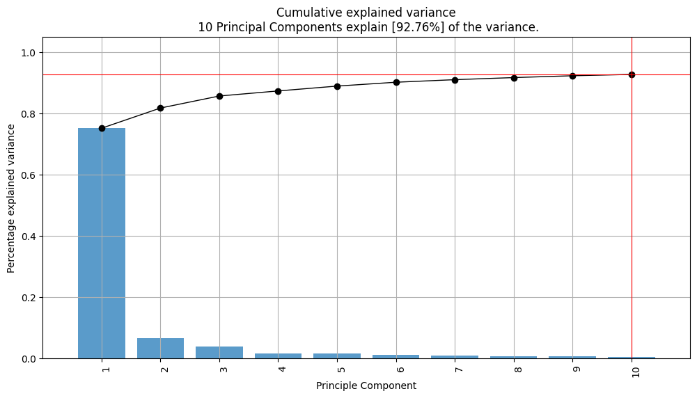
Using outlier detection method like the Hotelling T2 test and the squared prediction error (SPE/DmodX) just one outlier were found in the data which was decided to remain in data.
fig, axes = plt.subplots(ncols=2, figsize=(17,8))
ax1 = PCA_model.scatter(SPE=True, hotellingt2=True, cmap='tab10', ax=axes[0])
ax2 = PCA_model.biplot(SPE=True, hotellingt2=True, fontdict={'size': 8}, cmap='tab10', PC=[0,1,2], ax=axes[1])
plt.show()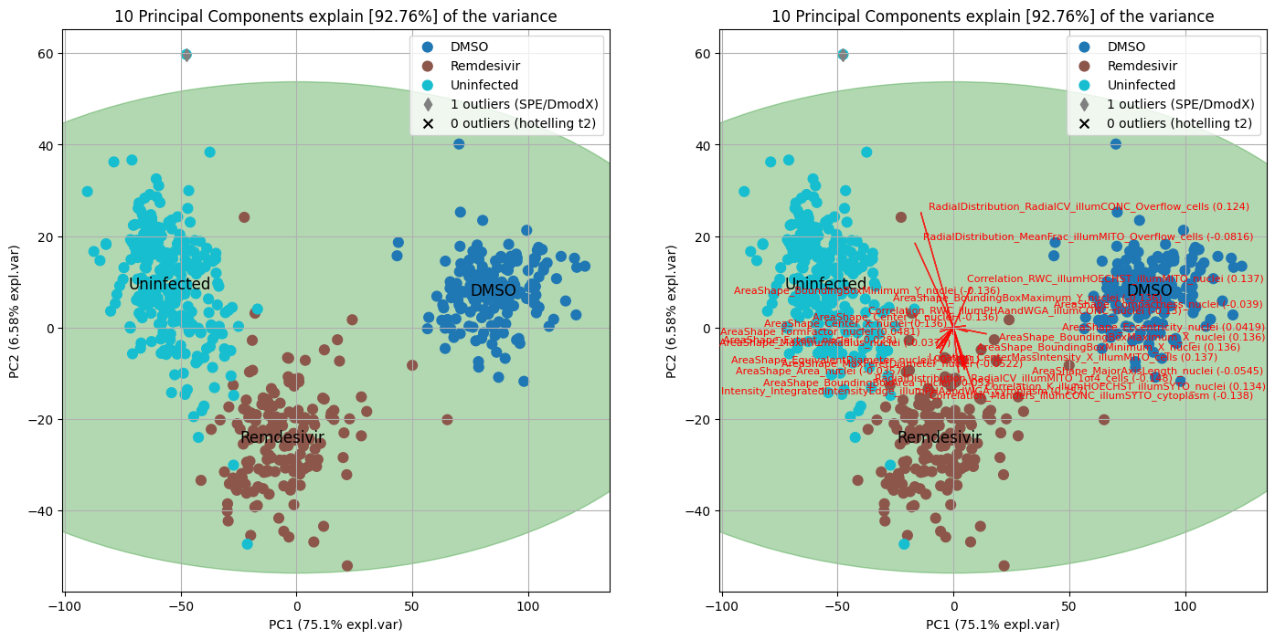
The loading values obtained from PCA were subsequently utilized as input for a k-means clustering algorithm, enabling the clustering of features according to their loadings. The idea is to find the features that provide same information and cluster them together. The process begins with the execution of PCA, which is then followed by the deployment of k-means clustering on the PCA loadings. This arrangement allows features to be clustered based on their loadings. This can be construed as their significance or contribution to the data variance then a new feature is calculated for every cluster. This feature represents the average of all features contained within that specific cluster.
def feature_reducer(df, feature_list, loading_dim=32, feat_output_dim=32):
import pandas as pd
from sklearn import preprocessing
from sklearn.decomposition import PCA
from sklearn.cluster import KMeans
df_dsmo_uninfected_remi = df.loc[(df['label'] == 'DMSO') | (df['label'] == 'Uninfected') | (df['label'] == 'Remdesivir')][feature_list]
X = df_dsmo_uninfected_remi.values
pca = PCA()
pca.fit(X)
loadings = pca.components_
loading_data = pd.DataFrame(loadings[:loading_dim]).T.values
# Perform k-means clustering
kmeans = KMeans(n_clusters=feat_output_dim, random_state=42, n_init=100).fit(loading_data)
# Get cluster assignments for each point
labels = kmeans.labels_
for i in range(feat_output_dim):
exec(f'f_{i+1}' + f'= loading_data[labels == {i}]')
f = pd.DataFrame({'features' : df_dsmo_uninfected_remi.columns.values, 'cluster': labels}).groupby("cluster").agg(list)
column_list = list(df.columns)
for feat in feature_list:
column_list.remove(feat)
new_df = df.loc[:,column_list].copy()
# new_df = df.loc[:,list(set(df.columns) - set(feature_list))].copy()
for i, f_list in enumerate(f['features']):
new_df[f'f{i+1}'] = df[f_list].apply(lambda x: x.mean() , axis=1)
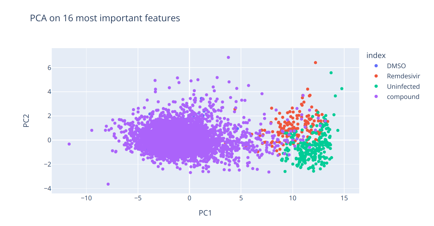
return new_df, fIn another approach to reduce the dimension, each feature’s ability to differentiate between the classes was evaluated by calculating the area of the triangle formed by the centroids of the classes in the feature space when we just use that specific feature and one highly related parameter to differentiate classes (for instance feature vs. number of nuclei) to plot all the points. For this, the centroids of the three distinct categories (‘Compound’, ‘Uninfected’, ‘Remdesivir’) for each feature ~ number of nuclei plot have been calculated. The area of the triangle formed by these centroids and the distance between them has been computed. This quantifies the separation between the three categories using each feature and helps to find the most descriptive feature. Features resulting in larger triangle areas were considered more informative.
import math
import numpy as np

def area_of_triangle(p1, p2, p3):
    # Calculate the length of each side of the triangle
    a = math.sqrt((p2[0] - p1[0])**2 + (p2[1] - p1[1])**2)
    b = math.sqrt((p3[0] - p2[0])**2 + (p3[1] - p2[1])**2)
    c = math.sqrt((p3[0] - p1[0])**2 + (p3[1] - p1[1])**2)

    # Calculate the semiperimeter of the triangle
    s = (a + b + c) / 2

    # Calculate the area using Heron's formula
    area = math.sqrt(s * (s - a) * (s - b) * (s - c))

    return area

def distance_between_centroids(centroid1, centroid2):
    # Calculate the distance using the distance formula
    distance = np.sqrt((centroid2[0] - centroid1[0])**2 + (centroid2[1] - centroid1[1])**2)

    return distance


scaler = preprocessing.StandardScaler(with_mean=True, with_std=True)
scaled_df = covid_df.copy()
scaled_df.loc[:, features] = scaler.fit_transform(scaled_df.loc[:, features])

scores = []
comp_remi = []
comp_uni = []
remi_uni = []
for feat in features[1:]:
    compound_coords = scaled_df.loc[scaled_df['label'] == 'compound',['Count_nuclei',feat]].values
    uninfected_coords = scaled_df.loc[scaled_df['label'] == 'Uninfected',['Count_nuclei',feat]].values
    remidesivir_coords = scaled_df.loc[scaled_df['label'] == 'Remdesivir',['Count_nuclei',feat]].values

    compound_centroid = np.mean(compound_coords, axis=0)
    uninfected_centroid = np.mean(uninfected_coords, axis=0)
    remidesivir_centroid = np.mean(remidesivir_coords, axis=0)

    area = area_of_triangle(compound_centroid, uninfected_centroid, remidesivir_centroid)
    comp_remi_dist =  distance_between_centroids(compound_centroid, remidesivir_centroid)
    comp_uni_dist =  distance_between_centroids(compound_centroid, uninfected_centroid)
    remi_uni_dist =  distance_between_centroids(remidesivir_centroid, uninfected_centroid)
    scores.append(area)
    comp_remi.append(comp_remi_dist)
    comp_uni.append(comp_uni_dist)
    remi_uni.append(remi_uni_dist)

feat_score = pd.DataFrame({'feat': features[1:],
                           'score': scores,
                           'comp_remi':comp_remi,
                           'comp_uni':comp_uni,
                           'remi_uni': remi_uni})
The features have been ranked based on the calculated area, seen as a measure of separation between the categories. The top 50 features have been selected. Between the first 50 features all annotated with MITO were removed because they bias our model. Therefore, 16 features remain as our selected features.
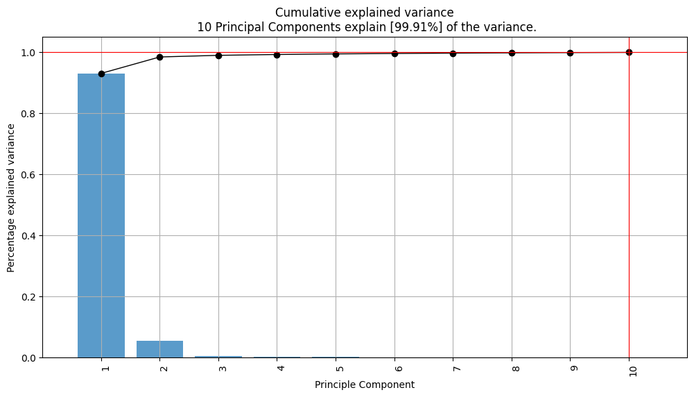
Finally, PCA has been performed again, this time exclusively on the selected features.
The PCA results demonstrate that the 10 principal components can now explain a very high percentage (99.91%) of the variance. The first principle component improved from describing 75.1 percent of variance to 93.0 percent. This indicates that the selected features capture most of the data variability. The value of PC1 was used for regression models as the target value.
2.1.1.3 Development of a binary classification of data
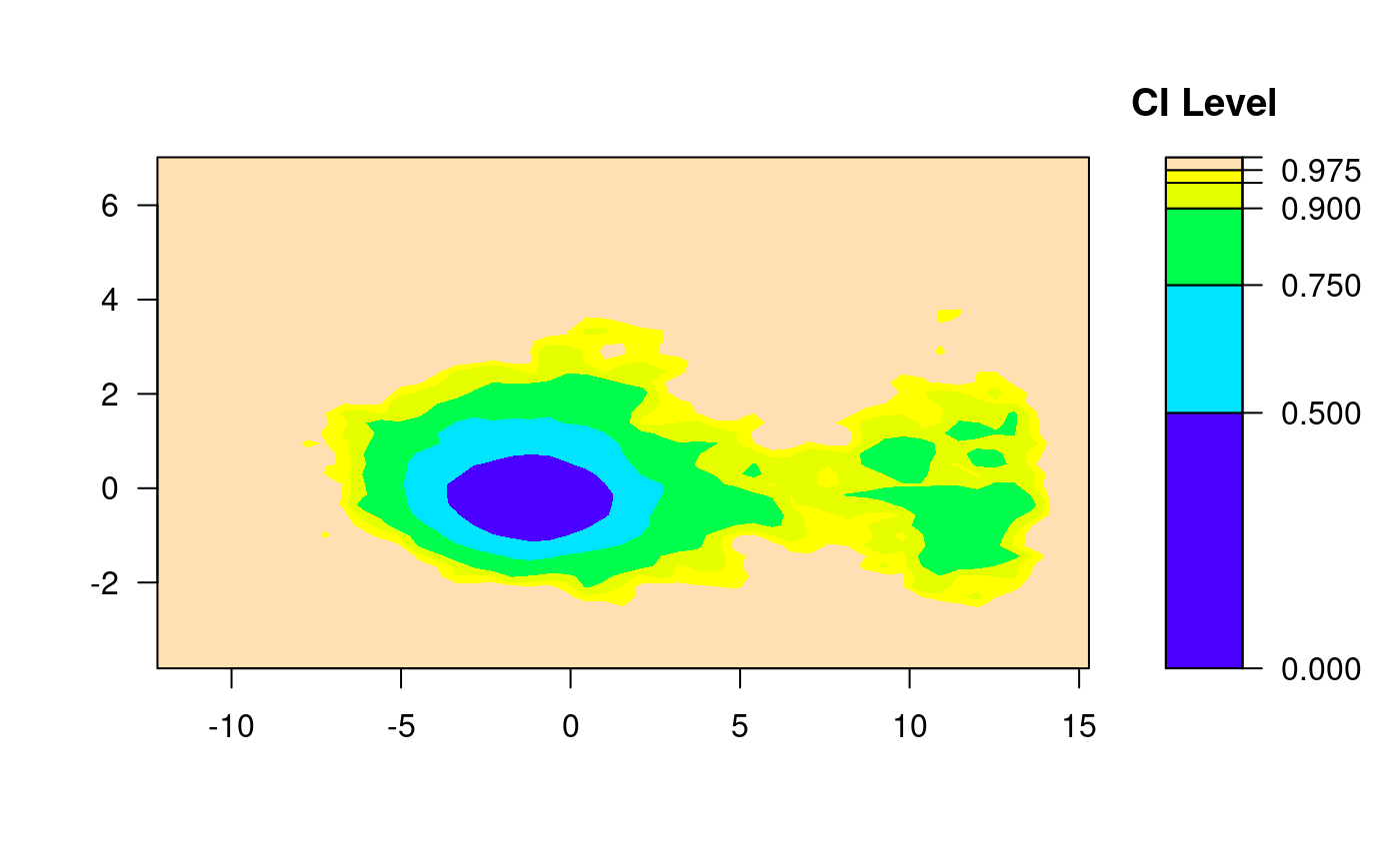
In this part, Kernel Density Estimation (KDE) and Empirical Confidence Regions (2d confidence intervals based on binned kernel density estimate) were utilized to inform the development of a binary classification model for identifying active and inactive compounds based on their PCA1 values.
Firstly, a two-dimensional KDE was performed on the compounds’ PCA1 and PCA2 values. This KDE plot provided a comprehensive understanding of the distribution of data points in the PCA space. It highlighted two distinct clusters corresponding to active and inactive compounds.
The KDE plot was further enhanced by overlaying empirical confidence regions on it. These regions were derived from the mean and covariance of the PCA1 and PCA2 values for each cluster. Two standard deviation ellipses were used, approximating 90% confidence regions for the location of the true mean of each cluster in the PCA space.
import numpy as np
import seaborn as sns
import matplotlib.pyplot as plt
from matplotlib.patches import Ellipse

mean1 = df_cluster1[['PC1', 'PC2']].mean()
cov1 = df_cluster1[['PC1', 'PC2']].cov()

mean2 = df_cluster2[['PC1', 'PC2']].mean()
cov2 = df_cluster2[['PC1', 'PC2']].cov()

fig, ax = plt.subplots(figsize=(7, 4))
# Draw the KDE plot
sns.kdeplot(data=df_clust, x='PC1', y='PC2', fill=True, ax=ax)

# Draw the confidence ellipses
for mean, cov in [(mean1, cov1), (mean2, cov2)]:
    eigenvalues, eigenvectors = np.linalg.eigh(cov)
    order = eigenvalues.argsort()[::-1]
    eigenvalues, eigenvectors = eigenvalues[order], eigenvectors[:, order]
    vx, vy = eigenvectors[:,0]
    theta = np.arctan2(vy, vx)

    # Draw a 2*2.146 ellipse for 90 % CI
    ellipse = Ellipse(xy=mean, width=2*2.146**np.sqrt(eigenvalues[0]),
                      height=2*2.146**np.sqrt(eigenvalues[1]),
                      angle=np.degrees(theta), edgecolor='red',
                      facecolor='none')
    ax.add_patch(ellipse)

plt.show()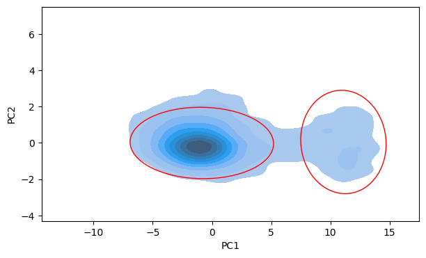
The intersection of these confidence regions was then examined. The PCA1 value of 5 at this intersection was hypothesized to be an effective threshold for binary classification of compounds. Any compound with a PCA1 value greater than this threshold was classified as ‘active’, and any compound with a PCA1 value less than this threshold was classified as ‘inactive’.
Importantly, this approach allowed the study to estimate a suitable classification threshold but also to visualize the uncertainty around this threshold and the potential overlap between the two classes. The method provided a data-driven way to set the classification threshold and offered insights into the inherent complexity of the data.
It should be noted that the assumptions of the Gaussian distribution and independent identically distributed data inherent to this method may not hold in all cases. Therefore, the results should be interpreted with caution. Further, the use of PCA1 values alone for classification may oversimplify the problem if the active and inactive compounds differ along other principal components as well. Therefore, additional analyses are recommended to validate and refine this binary classification model.
2.1.2 Compound, Protein and Pathway Data Aggregation
In the cell profiling data, the Simplified Molecular Input Line Entry System (SMILES) was incorporated to represent the chemical structure. The COVID-19 cell painting experiments that was carried out, was involved cell perturbations with over 5000 compounds. To uncover potential information regarding the protein binding capabilities and the pathways and assays in which these compounds are active, a highly recognized cross-reference annotation was necessitated.
The PubChem Chemical ID (CID) serves as an exhaustive cross-reference annotation for chemicals. The initial step involved the determination of the CIDs for all the chemical compounds. These identifiers were subsequently utilized for the aggregation of additional protein and pathway data. This approach facilitated finding the activity of the compounds within the biological systems.
import pubchempy as pcp

chemical_smiles = list(df['smiles'].values)

cids = []
for smiles in chemical_smiles:
    try:
        c = pcp.get_compounds(smiles, 'smiles')
        if c:
           cids.append(c[0].cid})
        else:
            print(f'No compound found for SMILES: {smiles}')
    except Exception as e:
        print(f'Error occurred: {e}')
The COVID-19 dataset consisted of compounds screened for potential activity against SARS-CoV-2. To analyze the associations between these compounds and proteins, an auxiliary dataset, sourced from the STITCH database, was utilized. The STITCH database provides information about interactions between chemicals and proteins. These connections were then indexed and collated to create a list of compounds with and their association with proteins.
Further, the connection between chemical compounds and their corresponding biological pathways was established through the following steps:
Initially, assay summaries for a selection of compounds were obtained from the PubChem database. These summaries provided information about various biological assays performed on the compounds, specifically emphasizing on the target gene IDs that interacted with the compounds during these assays. Only the assays reporting an ‘Active’ outcome and a non-empty target gene ID were retained for further analysis.
from io import StringIO
import polars as pl
import pubchempy as pcp

comp_gid = pl.read_csv('data/comp_gid.tsv', separator='\t')
cids = comp_gid.select(['pubchem_cid']).to_series().to_list()

cid_genid_df = pl.DataFrame(
  schema={'CID': pl.Int64, 'AID': pl.Int64, 'Target GeneID': pl.Utf8, 'Activity Value [uM]': pl.Float64, 'Assay Name': pl.Utf8}
  )

for cid in cids[:10]:
    try:
        csvStringIO = StringIO(pcp.get(cid, operation='assaysummary', output='CSV').decode("utf-8"))
        dictdf = pl.read_csv(csvStringIO, dtypes={'Activity Value [uM]': pl.Float64})
        ciddf = dictdf.filter(
          (pl.col("Activity Outcome") == "Active") & (pl.col("Target GeneID") != "")
          ).unique(
            subset='Target GeneID'
            ).select(
              ['CID', 'AID', 'Target GeneID', 'Activity Value [uM]',  'Assay Name']
              )
    except:
        ciddf = pl.DataFrame(
          schema={'CID': pl.Int64, 'AID': pl.Int64, 'Target GeneID': pl.Utf8, 'Activity Value [uM]': pl.Utf8, 'Assay Name': pl.Utf8}
          )

    cid_genid_df = cid_genid_df.vstack(ciddf)

cid_genid_df.write_csv('comp_geneid.tsv', separator='\t')
Subsequently, the list of unique target gene IDs was utilized to extract associated biological pathways from the PubChem database. These pathways, sourced from the WikiPathways database, link each gene ID to one or multiple biological pathways.
import polars as pl
import pubchempy as pcp

gene_id_list = cid_genid_df.select(pl.col('Target GeneID').cast(pl.Int64, strict=True)).unique(subset='Target GeneID', maintain_order=True).to_series().to_list()
genid_wpw_df = pl.DataFrame(schema={'Target GeneID': pl.Object, 'Wiki Pathway': pl.Utf8})

for gene_id in gene_id_list:
    try:
        ptw_list = pcp.get_json(gene_id, namespace='geneid', domain='gene', operation='pwaccs')['InformationList']['Information'][0]['PathwayAccession']
        wp = [i[13:] for i in list(filter(lambda x: 'WikiPathways' in x, ptw_list))]
        temp_df = pl.DataFrame({'Target GeneID':gene_id, 'Wiki Pathway': wp})
    except:
        temp_df = pl.DataFrame({'Target GeneID':gene_id, 'Wiki Pathway': ''})
    genid_wpw_df = genid_wpw_df.vstack(temp_df)


genid_wpw_df.write_csv('geneid_wpw.tsv', separator='\t')
Gene ID fetched from these databases can be converted to STITCH database annotation by using BIIT API:
import requests

r = requests.post(
    url='https://biit.cs.ut.ee/gprofiler/api/convert/convert/',
    json={
        'organism':'hsapiens',
        'target':'ENSP',
        'query':gene_id_list,
        'numeric_namespace': 'ENTREZGENE_ACC'
    }
    )
pl.DataFrame(r.json()['result']).select(['incoming', 'converted', 'name', 'description'])
Hence, a linkage from chemical compounds to biological pathways was constructed by associating compounds with target gene IDs from assays, and then connecting these gene IDs to biological pathways. This method of data preparation facilitated the exploration of potential mechanisms of action of compounds. It also provided an understanding of the biological processes potentially influenced by these compounds. It should be noted, however, that this is a simplified representation of the actual biological interactions, which are inherently more complex.
These curated lists of compounds, proteins, and pathways served as the foundation for constructing a multimodal graph. In this graph, the nodes represent compounds, proteins, and pathways while the edges depict the connections between them.
2.1.3 Featurizing the Biomedical Entities
In machine learning, featurization converts biomedical entities, which are often three-dimensional entities like chemicals and proteins, into a format that can be understood and processed by algorithms. Essentially, it involves converting the structure and properties into numerical vectors.
It is necessary because machine learning algorithms work with numerical data rather than understanding biological structures and properties directly. Featurization is accomplished through the application of different algorithm and ways which will be discussed in following section.
2.1.3.1 Featurizing Compounds
Starting with MACCS fingerprints, these are binary representations of a molecule based on the presence or absence of 167 predefined structural fragments. MACCS fingerprints are popular due to their simplicity, interpretability, and effectiveness at capturing structural information.
Morgan fingerprints, also known as circular fingerprints, are another type of molecular descriptor. They are generated by iteratively hashing the environments of atoms in a molecule. These fingerprints are characterized by their flexibility, as their radius and length can be adjusted. This allows for various levels of specificity in the representation of molecular structures.
import deepchem as dc

feat = dc.feat.CircularFingerprint(size=2048, radius=1)
morgan_fp = feat.featurize(smiles)
PubChem fingerprints are binary fingerprints consisting of 881 bits, each representing a particular chemical substructure or pattern. They were specifically designed for use with the PubChem database and provide detailed chemical structure encoding.
import pubchempy as pcp

cids = list(df.pubchem_cid[df['label']=='compound'])

bit_list = []
for cid in tqdm(cids):
    try:
        pubchem_compound =pcp.get_compounds(cid)[0]
        pubchem_fp = [int(bit) for bit in pubchem_compound.cactvs_fingerprint]
        bit_list.append(pubchem_fp)
    except:
        print(f'No PubChem FP found for {cid}')
        bit_list.append([])

pc_fp = np.asarray(bit_list)
The Mol2Vec fingerprint is inspired by the Word2Vec algorithm in Natural Language Processing. It considers molecules as sentences and SMILES as words, thus converting molecules into continuous vectors. This technique captures not only the presence of particular substructures but also their context within the molecule, providing a more nuanced representation.
In computational chemistry and drug discovery, molecules’ pre-treatment plays a crucial role in preparing them for machine learning applications. Molecules undergo optimization, where their 3D structure is refined and all possible conformations are explored. This step is vital as the 3D structure heavily influences various properties, such as reactivity and binding affinity. For Mordred and RDKit to compute all descriptors, we must optimize molecules and find their most energetically favorable conformations.
from rdkit import Chem
from rdkit.Chem import AllChem
from threading import active_count

num_thread = active_count()
def optimize_3d(mol, method):

    mol = Chem.AddHs(mol)
    # Generate initial 3D coordinates
    params = AllChem.ETKDG()
    params.useRandomCoords=True
    params.maxAttempts=5000
    AllChem.EmbedMolecule(mol, params)
    try:
        if method == 'MMFF':
            # optimize the 3D structure using the MMFF method (suitable for optimizing small to medium-sized molecules)
            AllChem.MMFFOptimizeMolecule(mol, maxIters=200, mmffVariant='MMFF94s')
        elif method == 'LOPT':
            # optimize the 3D structure using a combination of UFF and MMFF methods (can be used for optimizing larger and more complex molecules)
            # create a PyForceField object and set its parameters
            ff = AllChem.UFFGetMoleculeForceField(mol)
            ff.Initialize()
            ff.Minimize()
            AllChem.OptimizeMolecule(ff, maxIters=500)
        elif method == 'CONFOPT':
            # optimize each conformation using the PyForceField object (to explore the conformational space of a molecule and identify the most energetically favorable conformations)
            # generate 10 conformations using UFF
            # create a PyForceField object and set its parameters
            AllChem.EmbedMultipleConfs(mol, numConfs=10)
            ff = AllChem.UFFGetMoleculeForceField(mol)
            ff.Initialize()
            ff.Minimize()
            AllChem.OptimizeMoleculeConfs(mol, ff, maxIters=300, numThreads=num_thread)
        else:
            print(f"method should be from {['MMFF', 'LOPT', 'CONFOPT']}")
    except:
        pass
    return mol
RDKit descriptors include a comprehensive set of descriptors calculated directly from the molecule’s structure. These descriptors encompass a wide range of molecular properties, including size, shape, polarity, and topological characteristics. They are widely used in QSAR modeling and virtual screening applications due to their comprehensive nature.
from rdkit import Chem
from rdkit.Chem import Descriptors

# Define a function to calculate all the possible descriptors
def calculate_descriptors(smiles, idx):
    mol = Chem.MolFromSmiles(smiles)
    try:
        mol = optimize_3d(mol, 'LOPT')
    except:
        pass
    desc_lst = []
    for descriptor_name, descriptor_function in Descriptors.descList:
        try:
            descriptor_value = descriptor_function(mol)
            if descriptor_value == pd.notnull:
                print(f'No value for {descriptor_name}, output: {descriptor_value} for {idx}:{smiles}')
                desc_lst.append(np.nan)
            else:
                desc_lst.append(descriptor_value)
        except:
            pass
    return desc_lst

descriptor_list = []
for idx, sml in enumerate(tqdm(smiles)):
    compound_desc = calculate_descriptors(sml, idx)
    descriptor_list.append(compound_desc)

rdkit_desc_df = pd.DataFrame(descriptor_list, columns=[name for name, _ in Descriptors.descList]).astype(np.float64)
rdkit_desc_df = rdkit_desc_df.dropna(axis=1)
rdkit_desc = rdkit_desc_df.values.astype(np.float64)
Finally, Mordred descriptors provide a vast array of over 1600 three-dimensional, two-dimensional, and one-dimensional descriptors. These descriptors represent a wide variety of chemical information, ranging from simple atom counts and molecular weight to more complex descriptors such as electrotopological state indices and autocorrelation descriptors. The rich information provided by Mordred descriptors makes them an excellent choice for modeling complex molecular behaviors.
from mordred import Calculator, descriptors

molecules = [Chem.MolFromSmiles(sml) for sml in smiles]

# Define a function to calculate all the possible descriptors
def calculate_mordred_descriptors(mol, optimization= 'LOPT'):
    mol = optimize_3d(mol, optimization)
    # Create a Mordred calculator object
    calculator = Calculator(descriptors)
    return calculator(mol)

mdrd_descriptor_list = []
for idx, mol in enumerate(tqdm(molecules)):
    mol_desc = calculate_mordred_descriptors(mol)
    desc = list(mol_desc.asdict().values())
    mdrd_descriptor_list.append(desc)

mordred_desc_df = pd.DataFrame(mdrd_descriptor_list, columns=list(mol_desc.asdict().keys())).astype(np.float64)
mordred_desc_df = mordred_desc_df.dropna(axis=1)
mordred_desc = mordred_desc_df.values.astype(np.float64)
To summarize, the featureization process leverages multiple molecular descriptors to capture molecular structures’ complexity and diversity. Each descriptor contributes unique information about the molecule, resulting in a comprehensive and informative representation.
| Featurizing Technique | Description | Size | Binary | 3D Information | Adjustability |
|---|---|---|---|---|---|
| MACCS fingerprints | Predefined structural fragments | 167 | Yes | No | No |
| Morgan fingerprints (Circular fingerprints) | Hashing the environments of atoms in a molecule | Adjustable (2048 in the example) | Yes | No | Yes (Radius and length can be adjusted) |
| PubChem fingerprints | Chemical substructure or pattern | 881 | Yes | No | No |
| Mol2Vec fingerprint | SMILES as words | Variable | No | No | No |
| RDKit descriptors | Physico-chemical descriptors | >200 | No | Yes | No |
| Mordred descriptors | Physico-chemical descriptors | >1600 | No | Yes | No |
2.1.3.2 Featurizing Proteins
The transformation of protein sequences into embedding vectors using models pretrained on millions of proteins is highly beneficial. These models are trained to understand protein sequence patterns, structures, and dependencies. Thus, the resulting embeddings capture a wealth of information about protein sequences, including their evolutionary context, structural features, and biological functions.
BioTransformers is a Python package that provides a unified API to use and evaluate several pre-trained models for protein sequences. These models transform protein sequences into meaningful numerical representations, also known as embeddings. The extracted embeddings can then be used in downstream machine learning tasks such as protein classification, clustering, or prediction of protein properties.
The models you’ve selected, protbert and esm1_t34_670M_UR100, are two different pre-trained models available in BioTransformers.
ProtBert is a transformer-based model trained on a large corpus of protein sequences using a masked language modeling objective, similar to BERT models in natural language processing. The model’s architecture enables it to capture complex patterns and dependencies in the sequence data.
On the other hand, esm1_t34_670M_UR100 is part of the ESM (Evolutionary Scale Modeling) series of models, specifically trained on a large evolutionary scale of protein sequences. This model is designed to capture evolutionary patterns and sequence conservation information, which can be highly beneficial for protein-related tasks.
from biotransformers import BioTransformers
from tqdm.notebook import tqdm
import torch
import numpy as np
import pandas as pd
import pickle

def compute_embeddings(bio_trans, sequences, batch_size=10):
    embeddings = np.empty((0,1024), float)
    for idx in tqdm(range(0, len(sequences), batch_size)):
        batch = sequences[idx:idx+batch_size]
        embd = bio_trans.compute_embeddings(batch, pool_mode='mean', batch_size=batch_size, silent=True)['mean']
        embeddings = np.vstack((embeddings, embd))
    return embeddings

def save_embeddings(embeddings, filename):
    with open(filename, "wb") as f:
        pickle.dump(embeddings, f)

# Load sequences
seq_df = pd.read_csv('sequence.tsv', sep='\t')
sequences = list(seq_df['sequence'])

# Backends
backends = ["protbert", "esm1_t34_670M_UR100"]

for backend in backends:
      # Clear GPU memory
    torch.cuda.empty_cache()
    print(f"Processing with backend: {backend}")
    bio_trans = BioTransformers(backend, num_gpus=1)
    embeddings = compute_embeddings(bio_trans, sequences)
    save_embeddings(embeddings, f"{backend}_embeddings.pkl")
This rich representation can be leveraged in downstream tasks, improving the performance of various bioinformatics applications such as protein function prediction, protein-protein interaction prediction, and many others. By using pre-trained embeddings, one can also significantly reduce the computational cost and complexity associated with training deep learning models from scratch on large protein datasets.
2.1.3.3 Featurizing Pathways
BERT tokenizer from the Hugging Face Transformers library, a pre-trained model, was chosen for its ability to perform natural language processing tasks such as tokenization to vectorize biological pathways. This process involved splitting the text into individual tokens and encoding them as numerical IDs that could be understood by the BERT model. Padding and truncation techniques were applied to ensure consistent sequence lengths during tokenization. This step was critical as pathway descriptions often varied in length. By padding shorter sequences and truncating longer ones, uniformity was achieved.
This would simply allow the model recognize different pathways from each other.
from transformers import BertTokenizer

tokenizer = BertTokenizer.from_pretrained('bert-base-uncased')
string_list = pathway_df.select(pl.col('Wiki Pathway')).to_series().to_list()

# Tokenize the pathway descriptions
tokenized_strings = tokenizer(string_list, padding=True, truncation=True, return_tensors='pt')

# Retrieve the tokenized input IDs
pw_vector = tokenized_strings['input_ids']
2.1.4 COVID-19 Bio-Graph
Having all the data ready a multimodal graph was built that represents a complex network of interconnected biological entities - chemicals, proteins, and pathways. The graph contains 4,293 unique chemicals, each distinguished by a high-dimensional feature vector (4,272 features) that includes biochemical properties, SMILES strings, and phenotype features. The chemicals’ high-dimensional space has been condensed into a single feature PCA1 using dimensionality reduction techniques.
from torch_geometric.data import HeteroData

data = HeteroData()

data['chemical'].x = chemical_features.to(torch.float)                      # [num_chemicals, num_features_chemical]
data['chemical'].smiles = chemical_smiles                                   # [num_chemicals]
data['chemical'].y = chemical_y.long()                                      # [num_chemicals]
data['chemical'].pca1 = chemical_pca1.to(torch.float)                       # [num_chemicals]
data['chemical'].phenotype_feat = chemical_phenotype_feat.to(torch.float)   # [num_chemicals, 16]

for f, v in [('train', 'train'), ('valid', 'val'), ('test', 'test')]:
    idx = mask_df.select(
                ['connected_compound_gid', 'mask']
                ).filter(
                pl.col('mask') == f
                ).select('connected_compound_gid').to_numpy().flatten()
    idx = torch.from_numpy(idx)
    maskit = torch.zeros(data['chemical'].num_nodes, dtype=torch.bool)
    maskit[idx] = True
    data['chemical'][f'{v}_mask'] = maskit

data['protein'].x = protein_esm_embeddings.to(torch.float)  # [num_proteins, num_features_protein]
data['protein'].name = protein_names                        # [num_proteins]
data['protein'].seq = protein_sequences                     # [num_proteins]

data['pathway'].x = pathway_features.to(torch.float)        # [num_pathways, num_features_pathway]
data['pathway'].name = pathway_names                        # [num_pathways]

data['chemical', 'bind_to', 'protein'].edge_index = torch.from_numpy(compound_protein_deges).t().contiguous()     # [2, num_edges_bind]
data['pathway', 'activate_by', 'chemical'].edge_index = torch.from_numpy(pathway_compound_edges).t().contiguous() # [2, num_edges_activate]
data['protein', 'governs', 'pathway'].edge_index = torch.from_numpy(protein_pathway_edges).t().contiguous()       # [2, num_edges_govern]
The final output of this process was a HeteroData object from the PyTorch Geometric library, which represents a heterogeneous graph with various types of nodes and edges. This graph-based representation of the data encapsulates the interconnected nature of the compounds, proteins, and pathways, thereby providing a comprehensive overview of the interactions and associations within the COVID-19 cell profiling data.
Our multimodal graph, a complex mesh of interconnected biological entities, represents a wealth of relationships between chemicals, proteins, and pathways. It illustrates the intricate dynamics prevalent in molecular biology, serving as a robust framework for advanced modeling tasks.
Among the 4,293 chemicals, only 3,711 have known connections to at least one protein, whereas 1,376 chemicals are isolated, meaning they lack any known protein interactions. On the other hand, from the total of 16,733 proteins, 16,727 are known to interact with chemicals, leaving 2,839 proteins without any known chemical connections.
The graph also models 1,117 unique biological pathways. Only 282 proteins are known to govern these pathways. Interestingly, 3,220 chemicals are linked to all pathways, underscoring chemicals’ pervasive influence in biological processes. A distinct subset of 582 chemicals connect exclusively to pathways, without any protein connections, and 6 proteins have pathway connections but no compound connections.
Overall, the graph includes 4,293 chemicals and 16,733 proteins that have at least one known connection, either to proteins, pathways, or both. These connections, represented by the different types of edges, symbolize various biological interactions and regulatory mechanisms. The graph’s structure, supplemented by the additional attributes of each node type, provides a comprehensive data platform for downstream tasks.
The graph were further masked with training, validation, and testing subsets using a stratified approach to maintain a uniform distribution of classes across all subsets. This enabled the creation of robust machine learning models capable of effectively learning from training data and generalizing to unseen data.
2.1.5 Representing Chemical Molecules as Graph
In conventional drug discovery processes, chemical structures are often encoded as fixed-length feature vectors, which were explained in detail in the previous section (Featurizing). These vectors, while effective for some tasks, lack the nuanced structural information and context of the atoms and bonds within the molecule.
Recently, graph-based representations of molecules have gained popularity in computational chemistry and cheminformatics. In this approach, each molecule is represented as a graph, where atoms are considered as nodes and bonds as edges. This representation retains the context of the molecule, allowing for more sophisticated analysis and understanding of the molecular structure. Each atom (node) and bond (edge) can be associated with features such as atom type, bond type, atom hybridization, whether the bond is in a ring, etc. Graph convolutional networks (GCNs) can then be used to learn complex patterns from these graph-structured data.
The graph-based representation and the conventional vector-based representation each have their unique strengths. The graph representation can capture local structural information and long-range interactions in the molecule, while the vector-based representation can efficiently capture specific substructures or holistic properties like the physico-chemical characteristics of the molecule.
The initial step was to convert molecular structures into graph-based representations. This conversion was achieved using the MolGraphConvFeaturizer from the DeepChem library. This generated node and edge features considering additional aspects such as chirality and partial charge.
Two dataset classes were designed for classification task: CovidMolGraph_imbalance_classification and CovidMolGraph_balanced_classification. The imbalanced dataset will be used with weight on binary classes during the training. The balanced classification approach involved resampling the minority class in the training set to balance the class distribution, improving the model’s performance.These handled the unbalanced and balanced classifications of the dataset, respectively.
import os
import pickle
import torch
from typing import Callable, List, Optional
from sklearn import preprocessing
from tqdm import tqdm
import deepchem as dc
import polars as pl
from rdkit import Chem
import numpy as np
from sklearn.model_selection import train_test_split

from torch_geometric.data import (
    Data,
    Dataset,
    InMemoryDataset
)

class CovidMolGraph_imbalance_classification(InMemoryDataset):

    def __init__(self, root: str, transform: Optional[Callable] = None,
                 pre_transform: Optional[Callable] = None,
                 pre_filter: Optional[Callable] = None):
        super().__init__(root, transform, pre_transform, pre_filter)
        self.data, self.slices = torch.load(self.processed_paths[0])

    @property
    def processed_file_names(self) -> str:
        return 'covid_data_processed.pt'

    def process(self):
        df = pl.read_csv('covid_20230504.tsv', separator='\t').filter(
            pl.col('label') == 'compound'
        ).with_columns(
            pl.col('pca1').apply(lambda x: 1 if x >= 5 else 0).alias('activity')
        ).with_columns(
            pl.lit([i for i in range(5087)]).alias('xid')
        )

        with open("all_feat.pkl", "rb") as f:
            chemical_features = pickle.load(f)

        phenotype_features = df.columns[5:-6]
        smiles = df.select(['pubchem_smiles']).to_numpy().flatten()
        y = df.select(['activity']).to_numpy().flatten()
        pca1 = df.select(['pca1']).to_numpy().flatten()

        # Convert the smiles into numerical features using a featurizer from deepchem
        # Using MolGraphConvFeaturizer
        featurizer = dc.feat.MolGraphConvFeaturizer(use_edges=True, use_chirality= True, use_partial_charge=True)
        graphs = featurizer.featurize(smiles, y=y)

        data_list = []
        for idx, graph in tqdm(enumerate(graphs)):
            edge_features = torch.from_numpy(graph.edge_features).float()
            g = Data(x=torch.from_numpy(graph.node_features).float(),
                            edge_index=torch.from_numpy(graph.edge_index).long(),
                            edge_attr=edge_features,
                            y=torch.tensor(y[idx]).long().unsqueeze(0),
                            chem_features=torch.from_numpy(chemical_features[idx]).float().unsqueeze(0),
                            smiles=smiles[idx])
            data_list.append(g)

            if self.pre_filter is not None:
                data_list = [data for data in data_list if self.pre_filter(data)]

            if self.pre_transform is not None:
                data_list = [self.pre_transform(data) for data in data_list]

        data, slices = self.collate(data_list)
        torch.save((data, slices), self.processed_paths[0])

class CovidMolGraph_balanced_classification(InMemoryDataset):

    def __init__(self, root: str, transform: Optional[Callable] = None,
                 pre_transform: Optional[Callable] = None,
                 pre_filter: Optional[Callable] = None):
        super().__init__(root, transform, pre_transform, pre_filter)
        self.data, self.slices = torch.load(self.processed_paths[0])

    @property
    def processed_file_names(self) -> str:
        return 'covid_data_processed.pt'

    def process(self):
        df = pl.read_csv('covid_20230504.tsv', separator='\t').filter(
            pl.col('label') == 'compound'
        ).with_columns(
            pl.col('pca1').apply(lambda x: 1 if x >= 5 else 0).alias('activity')
        ).with_columns(
            pl.lit([i for i in range(5087)]).alias('xid')
        )

        with open("all_feat.pkl", "rb") as f:
            chemical_features = pickle.load(f)

        phenotype_features = df.columns[5:-6]
        smiles = df.select(['pubchem_smiles']).to_numpy().flatten()
        y = df.select(['activity']).to_numpy().flatten()
        pca1 = df.select(['pca1']).to_numpy().flatten()

        # Example data with 4 classes
        data = pca1
        labels = y

        # Split the data into train, validation, and test sets
        train_data, val_data, train_labels, val_labels = train_test_split(data, labels, test_size=1000, random_state=42,
                                                                          stratify=labels)
        train_list = ['train' for _ in range(4087)]
        val_list = ['valid' for _ in range(1000)]
        mask_list = train_list + val_list

        mask = pl.DataFrame(
            {
                'pca1': np.hstack((train_data, val_data)),
                'mask': mask_list
            }
        ).sort('pca1', descending=True)
        df = df.join(mask, on='pca1', how='left')

        neg_class = df["activity"].value_counts()[0]['counts'].item()
        pos_class = df["activity"].value_counts()[1]['counts'].item()
        multiplier = int(neg_class/pos_class) - 1

        df = df.with_columns(
            pl.col('activity').apply(lambda x: x*multiplier if x == 1 else 1).alias('to_replicate')
        )

        train_df = df.filter(pl.col('mask') == 'train')
        valid_df = df.filter(pl.col('mask') == 'valid')

        balanced_train_df = train_df.select(
            pl.exclude('to_replicate').repeat_by('to_replicate').explode()
        )
        balanced_valid_df = valid_df.select(
            pl.exclude('to_replicate').repeat_by('to_replicate').explode()
        )
        balanced_df = balanced_train_df.vstack(balanced_valid_df).sort("xid", descending=False)
        index_to_replicate = balanced_df.groupby("xid", maintain_order=True).count()['count'].to_numpy()

        balanced_chemical_features = np.repeat(chemical_features, index_to_replicate, axis=0)
        balanced_smiles = balanced_df.select(['pubchem_smiles']).to_series().to_list()
        balanced_y = balanced_df.select(['activity']).to_numpy().flatten()
        balanced_pca1 = balanced_df.select(['pca1']).to_numpy().flatten()

        # Convert the smiles into numerical features using a featurizer from deepchem
        # Using MolGraphConvFeaturizer
        featurizer = dc.feat.MolGraphConvFeaturizer(use_edges=True, use_chirality= True, use_partial_charge=True)
        graphs = featurizer.featurize(balanced_smiles, y=balanced_y)

        data_list = []
        for idx, graph in tqdm(enumerate(graphs)):
            edge_features = torch.from_numpy(graph.edge_features).float()
            g = Data(x=torch.from_numpy(graph.node_features).float(),
                            edge_index=torch.from_numpy(graph.edge_index).long(),
                            edge_attr=edge_features,
                            y=torch.tensor(balanced_y[idx]).long().unsqueeze(0),
                            chem_features=torch.from_numpy(balanced_chemical_features[idx]).float().unsqueeze(0),
                            smiles=balanced_smiles[idx])
            data_list.append(g)

            if self.pre_filter is not None:
                data_list = [data for data in data_list if self.pre_filter(data)]

            if self.pre_transform is not None:
                data_list = [self.pre_transform(data) for data in data_list]

        data, slices = self.collate(data_list)
        torch.save((data, slices), self.processed_paths[0])
Another two dataset also were created for regression task. The difference is that the model target y instead of binary classification of active and inactive compound would be the molecule PCA1 value.
class CovidMolGraph_imbalance_regression(InMemoryDataset):

    def __init__(self, root: str, transform: Optional[Callable] = None,
                 pre_transform: Optional[Callable] = None,
                 pre_filter: Optional[Callable] = None):
        super().__init__(root, transform, pre_transform, pre_filter)
        self.data, self.slices = torch.load(self.processed_paths[0])

    @property
    def processed_file_names(self) -> str:
        return 'covid_data_processed.pt'

    def process(self):
        df = pl.read_csv('covid_20230504.tsv', separator='\t').filter(
            pl.col('label') == 'compound'
        ).with_columns(
            pl.col('pca1').apply(lambda x: 1 if x >= 5 else 0).alias('activity')
        ).with_columns(
            pl.lit([i for i in range(5087)]).alias('xid')
        )

        with open("all_feat.pkl", "rb") as f:
            chemical_features = pickle.load(f)

        phenotype_features = df.columns[5:-6]
        smiles = df.select(['pubchem_smiles']).to_numpy().flatten()
        y = df.select(['activity']).to_numpy().flatten()
        pca1 = df.select(['pca1']).to_numpy().flatten()

        # Convert the smiles into numerical features using a featurizer from deepchem
        # Using MolGraphConvFeaturizer
        featurizer = dc.feat.MolGraphConvFeaturizer(use_edges=True, use_chirality= True, use_partial_charge=True)
        graphs = featurizer.featurize(smiles, y=pca1)

        data_list = []
        for idx, graph in tqdm(enumerate(graphs)):
            edge_features = torch.from_numpy(graph.edge_features).float()
            g = Data(x=torch.from_numpy(graph.node_features).float(),
                            edge_index=torch.from_numpy(graph.edge_index).long(),
                            edge_attr=edge_features,
                            y=torch.tensor(pca1[idx]).long().unsqueeze(0),
                            chem_features=torch.from_numpy(chemical_features[idx]).float().unsqueeze(0),
                            smiles=smiles[idx])
            data_list.append(g)

            if self.pre_filter is not None:
                data_list = [data for data in data_list if self.pre_filter(data)]

            if self.pre_transform is not None:
                data_list = [self.pre_transform(data) for data in data_list]

        data, slices = self.collate(data_list)
        torch.save((data, slices), self.processed_paths[0])

class CovidMolGraph_balanced_regression(InMemoryDataset):

    def __init__(self, root: str, transform: Optional[Callable] = None,
                 pre_transform: Optional[Callable] = None,
                 pre_filter: Optional[Callable] = None):
        super().__init__(root, transform, pre_transform, pre_filter)
        self.data, self.slices = torch.load(self.processed_paths[0])

    @property
    def processed_file_names(self) -> str:
        return 'covid_data_processed.pt'

    def process(self):
        df = pl.read_csv('covid_20230504.tsv', separator='\t').filter(
            pl.col('label') == 'compound'
        ).with_columns(
            pl.col('pca1').apply(lambda x: 1 if x >= 5 else 0).alias('activity')
        ).with_columns(
            pl.lit([i for i in range(5087)]).alias('xid')
        )

        with open("all_feat.pkl", "rb") as f:
            chemical_features = pickle.load(f)

        phenotype_features = df.columns[5:-6]
        smiles = df.select(['pubchem_smiles']).to_numpy().flatten()
        y = df.select(['activity']).to_numpy().flatten()
        pca1 = df.select(['pca1']).to_numpy().flatten()

        # Example data with 4 classes
        data = pca1
        labels = y

        # Split the data into train, validation, and test sets
        train_data, val_data, train_labels, val_labels = train_test_split(data, labels, test_size=1000, random_state=42,
                                                                          stratify=labels)
        train_list = ['train' for _ in range(4087)]
        val_list = ['valid' for _ in range(1000)]
        mask_list = train_list + val_list

        mask = pl.DataFrame(
            {
                'pca1': np.hstack((train_data, val_data)),
                'mask': mask_list
            }
        ).sort('pca1', descending=True)
        df = df.join(mask, on='pca1', how='left')

        neg_class = df["activity"].value_counts()[0]['counts'].item()
        pos_class = df["activity"].value_counts()[1]['counts'].item()
        multiplier = int(neg_class/pos_class) - 1

        df = df.with_columns(
            pl.col('activity').apply(lambda x: x*multiplier if x == 1 else 1).alias('to_replicate')
        )

        train_df = df.filter(pl.col('mask') == 'train')
        valid_df = df.filter(pl.col('mask') == 'valid')

        balanced_train_df = train_df.select(
            pl.exclude('to_replicate').repeat_by('to_replicate').explode()
        )
        balanced_valid_df = valid_df.select(
            pl.exclude('to_replicate').repeat_by('to_replicate').explode()
        )
        balanced_df = balanced_train_df.vstack(balanced_valid_df).sort("xid", descending=False)
        index_to_replicate = balanced_df.groupby("xid", maintain_order=True).count()['count'].to_numpy()

        balanced_chemical_features = np.repeat(chemical_features, index_to_replicate, axis=0)
        balanced_smiles = balanced_df.select(['pubchem_smiles']).to_series().to_list()
        balanced_y = balanced_df.select(['activity']).to_numpy().flatten()
        balanced_pca1 = balanced_df.select(['pca1']).to_numpy().flatten()

        # Convert the smiles into numerical features using a featurizer from deepchem
        # Using MolGraphConvFeaturizer
        featurizer = dc.feat.MolGraphConvFeaturizer(use_edges=True, use_chirality= True, use_partial_charge=True)
        graphs = featurizer.featurize(balanced_smiles, y=balanced_pca1)

        data_list = []
        for idx, graph in tqdm(enumerate(graphs)):
            edge_features = torch.from_numpy(graph.edge_features).float()
            g = Data(x=torch.from_numpy(graph.node_features).float(),
                            edge_index=torch.from_numpy(graph.edge_index).long(),
                            edge_attr=edge_features,
                            y=torch.tensor(balanced_pca1[idx]).long().unsqueeze(0),
                            chem_features=torch.from_numpy(balanced_chemical_features[idx]).float().unsqueeze(0),
                            smiles=balanced_smiles[idx])
            data_list.append(g)

            if self.pre_filter is not None:
                data_list = [data for data in data_list if self.pre_filter(data)]

            if self.pre_transform is not None:
                data_list = [self.pre_transform(data) for data in data_list]

        data, slices = self.collate(data_list)
        torch.save((data, slices), self.processed_paths[0])
2.2 Models
2.2.1 Graph-Level Molecular Predictor (GLMP)
This model operates at the level of the graph, predicting properties based on the structural features of molecules. In machine learning applications in chemistry, compound representation plays a crucial role. The traditional approach involves converting chemical compounds into numerical vectors using various algorithms. However, a new popular alternative approach is molecule graph representation. This treats the compound as a graph structure with atoms as nodes and bonds as edges. This method captures atom connectivity and spatial arrangement within the molecule, providing more detailed information.
Conversely, the conventional vector conversion method transforms chemical compounds into fixed-length vectors by encoding molecular descriptors or fingerprints. Molecular descriptors encompass essential chemical properties, while fingerprints encode the presence or absence of specific substructures within the compound. Although vector representations are more concise and compatible with traditional machine learning algorithms, molecule graphs offer enhanced versatility and applicability to various chemistry tasks. Graph representations’ ability to leverage connectivity patterns and atom-level information leads to improved predictive performance and a deeper understanding of chemical phenomena.
When comparing the two approaches, molecule graphs excel at explicitly capturing structural information and atom relationships, making them advantageous for tasks reliant on spatial arrangement or connectivity patterns. On the other hand, conventional vector representations are more compact and suitable for traditional machine learning algorithms, making them preferable for larger datasets or tasks that don’t require explicit structural information. Molecule graphs can handle inputs of variable sizes, accommodating molecules with different atom numbers, whereas vector representations typically require fixed-size inputs. However, vector representations may sacrifice some fine-grained structural details or substructure information that molecule graphs can capture.
The GLMP (Graph-Level Molecular Predictor) model is designed to leverage both molecular graph representations and conventional vector representations in its architecture. The model combines the strengths of both approaches to enhance predictive performance and capture detailed structural information.
import torch
import torch.nn.functional as F
from torch.nn import Linear, BatchNorm1d, ModuleList
from torch_geometric.nn import TransformerConv, TopKPooling
from torch_geometric.nn import global_mean_pool as gap, global_max_pool as gmp

torch.manual_seed(42)
device = torch.device('cuda' if torch.cuda.is_available() else 'cpu')

class GLMP(torch.nn.Module):
    def __init__(self, feature_size, model_params):
        super(GNN, self).__init__()
        embedding_size = model_params["model_embedding_size"]
        n_heads = model_params["model_attention_heads"]
        self.n_layers = model_params["model_layers"]
        dropout_rate = model_params["model_dropout_rate"]
        top_k_ratio = model_params["model_top_k_ratio"]
        self.top_k_every_n = model_params["model_top_k_every_n"]
        dense_neurons = model_params["model_dense_neurons"]
        edge_dim = 11

        self.conv_layers = ModuleList([])
        self.transf_layers = ModuleList([])
        self.pooling_layers = ModuleList([])
        self.bn_layers = ModuleList([])

        # Transformation layer
        self.conv1 = TransformerConv(feature_size,
                                    embedding_size,
                                    heads=n_heads,
                                    dropout=dropout_rate,
                                    edge_dim=edge_dim,
                                    beta=True)

        self.transf1 = Linear(embedding_size*n_heads, embedding_size)
        self.bn1 = BatchNorm1d(embedding_size)
        self.bn2 = BatchNorm1d(8192)
        self.bn3 = BatchNorm1d(4096)
        self.bn4 = BatchNorm1d(2048)


        # Other layers
        for i in range(self.n_layers):
            self.conv_layers.append(TransformerConv(embedding_size,
                                                    embedding_size,
                                                    heads=n_heads,
                                                    dropout=dropout_rate,
                                                    edge_dim=edge_dim,
                                                    beta=True))

            self.transf_layers.append(Linear(embedding_size*n_heads, embedding_size))
            self.bn_layers.append(BatchNorm1d(embedding_size))
            if i % self.top_k_every_n == 0:
                self.pooling_layers.append(TopKPooling(embedding_size, ratio=top_k_ratio))


        # Linear layers
        self.linear1 = Linear(4784, 8192)
        self.linear2 = Linear(8192, 4096)
        self.linear3 = Linear(4096, 2048)
        self.linear4 = Linear(2048, 1)


    def forward(self, data):
        x, edge_attr, edge_index, batch_index, chem_features = data.x, data.edge_attr, data.edge_index, data.batch, data.chem_features
        # Initial transformation
        x = self.conv1(x, edge_index, edge_attr)
        x = torch.relu(self.transf1(x))
        x = self.bn1(x)

        # Holds the intermediate graph representations
        global_representation = []

        for i in range(self.n_layers):
            x = self.conv_layers[i](x, edge_index, edge_attr)
            x = torch.relu(self.transf_layers[i](x))
            x = self.bn_layers[i](x)
            # Always aggregate last layer
            if i % self.top_k_every_n == 0 or i == self.n_layers:
                x , edge_index, edge_attr, batch_index, _, _ = self.pooling_layers[int(i/self.top_k_every_n)](
                    x, edge_index, edge_attr, batch_index
                    )
                # Add current representation
                global_representation.append(torch.cat([gmp(x, batch_index), gap(x, batch_index)], dim=1))

        x = sum(global_representation)
        # chem_features concatenated with graph-level representations
        x = torch.cat([x, chem_features], dim=1)

        # Output block
        x = torch.relu(self.linear1(x))
        x = F.dropout(x, p=0.7, training=self.training)
        x = self.bn2(x)
        x = torch.relu(self.linear2(x))
        x = F.dropout(x, p=0.7, training=self.training)
        x = self.bn3(x)
        x = self.linear3(x)
        x = F.dropout(x, p=0.7, training=self.training)
        x = self.bn4(x)
        x = self.linear4(x)

        return x
The core of the GLMP model is a graph neural network (GNN) implemented using PyTorch. The GNN takes molecular graphs as input and applies a series of graph convolutional layers to capture atom connectivity and spatial arrangement within the molecules. The graph convolutional layers are implemented using a variant of the Transformer architecture, called TransformerConv, which incorporates attention mechanisms to capture global dependencies.
In addition to the graph convolutional layers, the GLMP model also includes traditional linear layers for further processing and prediction. These linear layers operate on the representations obtained from the graph convolutional layers and other features, such as chemical descriptors or fingerprints encoded as fixed-length vectors.
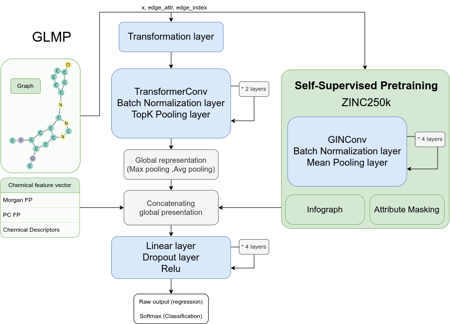
Graph-Level Molecular Predictor (GLMP) model architecture. GLMP implements a graph neural network, treating molecules as graph structures for detailed connectivity and spatial arrangement analysis. Combined with conventional numerical chemical vectors, GLMP performs graph-level molecular property prediction.
The GLMP model consists of the following components:
Graph Convolutional Layers: The model uses multiple graph convolutional layers, implemented as instances of the TransformerConv class, to capture structural information from the molecule graphs. These layers perform graph convolutions, incorporating attention mechanisms and edge features to enhance the model’s ability to capture atom relationships.
Linear and Batch Normalization Layers: After each graph convolutional layer, the GLMP model applies linear transformations followed by batch normalization to further process the representations obtained. These layers help refine the representations and make them suitable for downstream tasks.
Pooling Layers: The GLMP model includes pooling layers, specifically the TopKPooling class, which aggregates the node representations at certain intervals. The pooling layers help to condense the graph-level information and capture important features.
Chemical Features: The GLMP model incorporates additional chemical features, such as molecular descriptors or fingerprints, encoded as fixed-length vectors. These features are concatenated with graph-level representations at a later stage of the model.
Final Linear Layers: The GLMP model concludes with a series of linear layers, which further process the combined representations of the graph-level information and the additional chemical features. These layers progressively reduce the dimensionality of the representations and eventually output a single value for prediction.
By combining graph convolutional layers, linear layers, pooling layers, and chemical features, the GLMP model can effectively capture the detailed structural information present in molecular graphs. This allows the model to handle inputs of variable sizes, accommodate different atom numbers, and make predictions based on both spatial arrangement and essential chemical properties.
2.2.2 Bio-Graph Integrative Classifier/Regressor (BioGIC/BioGIR)
2.2.2.1 Classification/Regression
The Bio-Graph Integrative Classifier/Regressor (BioGIC/BioGIR) is envisioned as a model that assimilates information from the COVID-19 Bio-Graph, a complex network encapsulating different biological entities, such as chemical compounds, proteins, and pathways. This model performs classification or regression tasks based on the intricate relationships and interactions among these biological entities alongside the biological entities’ feature vectors.
The COVID-19 Bio-Graph allows for a more comprehensive representation of interdependencies. The proposed BioGIC/BioGIR model aims to leverage this wealth of information combined with feature vectors that represent the relevant information about the nodes they represent. This is to predict the properties or behaviors of certain entities, such as identifying active chemical compounds.
The BioGIC/BioGIR model architecture could be based upon a combination of different Graph Convolution Networks (GCNs). Graph Attention Network (GAT) convolution layer, is usually used for capturing the local neighborhood relationships of the nodes. GAT layer provides an attention mechanism allowing the model to weigh neighbor nodes differently based on their importance. Also, a sequence of Relational Graph Convolutional Network (RGCN) layers could be particularly beneficial for heterogeneous graphs, which are graphs with different types of nodes and edges. RGCN layers can learn separate weights for different types of edges, thereby modeling different types of relationships more accurately. GraphSAGE is another GCN that is a suitable general-purpose graph convolution operation and works reasonably well in many scenarios. It’s capable of generating embeddings for unseen data, which is an advantage if you expect to be working with active compounds that weren’t in your training data. However, it treats all neighbor nodes equally when aggregating their features, which might not be ideal in a heterogeneous graph where different types of nodes could have different importance.
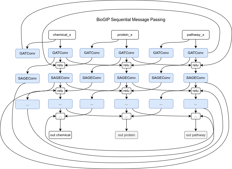
For BioGIP to be able to operate on heterogeneous graphs we have to duplicate the model’s message functions to cater to each unique edge type. As a result, the updated model expects dictionaries of all node and edge types, instead of single tensors that homogeneous graphs use. This adjustment enables message passing in multi-partite graphs by passing a set of input to the different convolutional layers. For simplicity only the BioGIP for sequential message passing is depicted here but the idea is the same for any complex architecture.
The model would also include appropriate optimization techniques and loss functions suitable for the task at hand. For a classification task, a cross-entropy loss function would be used, while for regression tasks, mean squared error or another suitable loss function could be employed. The training process would involve backpropagation and optimization of the weights to minimize the loss function.
The BioGIC/BioGIR model, by virtue of its design, allows for the integration of the complex relationships among various biological entities present in the COVID-19 Bio-Graph.
The decision to concatenate embeddings from each layer via a pooling mechanism versus passing messages serially through the layers depends on the specific task and data. Both approaches have their strengths and weaknesses, and they capture different types of information.
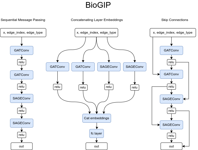
The BioGIP model design can consider sequential layer information passing for abstract representation tasks, layer embedding concatenation to preserve multi-scale graph information, or the use of skip or residual connections to maintain information flow and address the vanishing gradient issue in deeper models.
- Passing Messages in Series: This approach sequentially passes information through layers, with each layer potentially transforming and aggregating the information from the previous layer. This approach might be better suited if the task requires more abstract representations, as the information is aggregated and transformed across layers. However, one potential drawback is that information from the initial layers could be lost or diluted in this process.
from torch_geometric.nn import GATConv, RGCNConv, SAGEConv

class BioGI(torch.nn.Module):
    def __init__(self, hidden_channels, out_channels):
        super().__init__()
        self.conv1 = GATConv((-1, -1), hidden_channels)
        self.conv2 = SAGEConv(hidden_channels, hidden_channels)
        self.conv3 = RGCNConv(hidden_channels, hidden_channels, num_relations=dataset.num_relations, num_bases=10)
        self.conv4 = RGCNConv(hidden_channels, out_channels, num_relations=dataset.num_relations, num_bases=10)

    def forward(self, x, edge_index, edge_type):
        x = self.conv1(x, edge_index).relu()
        x = self.conv2(x, edge_index).relu()
        x = self.conv3(x, edge_index, edge_type).relu()
        x = self.conv4(x, edge_index, edge_type)
        return F.log_softmax(x, dim=1)

model = BioGI(hidden_channels=32, out_channels=dataset.num_classes)
model = to_hetero(model, data.metadata(), aggr='sum')- Concatenating Layer Embeddings: This approach can be beneficial as it allows the model to preserve and learn from information at different levels of abstraction. Each layer in a Graph Neural Network captures different types of information - initial layers capture local information, while deeper layers aggregate information from a larger neighborhood. Concatenating these embeddings can help the model leverage all this information simultaneously. Pooling mechanisms can be used to reduce dimensionality if needed. This approach might work well if the relevant information for the task is spread across different scales of the graph.
from torch_geometric.nn import GATConv, RGCNConv, SAGEConv
from torch.nn import Linear

class BioGI(torch.nn.Module):
    def __init__(self, hidden_channels, out_channels):
        super().__init__()
        self.conv1 = GATConv((-1, -1), hidden_channels)
        self.conv2 = SAGEConv(hidden_channels, hidden_channels)
        self.conv3 = RGCNConv(hidden_channels, hidden_channels, num_relations=dataset.num_relations, num_bases=10)
        self.conv4 = RGCNConv(hidden_channels, out_channels, num_relations=dataset.num_relations, num_bases=10)
        self.fc = Linear(hidden_channels*4, out_channels) # Fully connected layer

    def forward(self, x, edge_index, edge_type):
        x1 = self.conv1(x, edge_index).relu()
        x2 = self.conv2(x1, edge_index).relu()
        x3 = self.conv3(x2, edge_index, edge_type).relu()
        x4 = self.conv4(x3, edge_index, edge_type).relu()

        x = torch.cat([x1, x2, x3, x4], dim=-1)  # Concatenate along the last dimension
        x = self.fc(x)  # Pass through the fully connected layer
        return F.log_softmax(x, dim=1)

model = BioGI(hidden_channels=32, out_channels=dataset.num_classes)
model = to_hetero(model, data.metadata(), aggr='sum')- Skip connections or residual connections: Skip connections, also known as residual connections, are a technique used in deep neural networks to combat the vanishing gradient problem and to ease the training of deeper models. Skip connections work by adding the input to a layer to its output rather than directly feeding its output into the next layer. Through this approach, it is possible to maintain the flow of information and gradients through the network, thus making it easier to train deeper models. This is because during backpropagation, the gradients have a direct path through the skip connections, helping to mitigate the vanishing gradient problem where gradients can become very small and training can become difficult.
from torch_geometric.nn import GATConv, RGCNConv, SAGEConv
from torch.nn import Linear

class BioGI(torch.nn.Module):
    def __init__(self, hidden_channels, out_channels):
        super().__init__()
        self.conv1 = GATConv((-1, -1), hidden_channels)
        self.conv2 = SAGEConv(hidden_channels, hidden_channels)
        self.conv3 = RGCNConv(hidden_channels, hidden_channels, num_relations=dataset.num_relations, num_bases=10)
        self.conv4 = RGCNConv(hidden_channels, out_channels, num_relations=dataset.num_relations, num_bases=10)
        self.skip = Linear(hidden_channels, out_channels)  # Skip connection

    def forward(self, x, edge_index, edge_type):
        x1 = self.conv1(x, edge_index).relu()
        x2 = self.conv2(x1, edge_index).relu() + x1
        x3 = self.conv3(x2, edge_index, edge_type).relu() + self.skip(x2)
        x4 = self.conv4(x3, edge_index, edge_type).relu() + self.skip(x3)
        return F.log_softmax(x4, dim=1)

model = BioGI(hidden_channels=32, out_channels=dataset.num_classes)
model = to_hetero(model, data.metadata(), aggr='sum')
It’s difficult to say definitively which approach is more effective in this case without empirical testing. Both approaches could work well, and their performance may vary depending on the specifics of the data and task. It could be beneficial to implement both approaches and conduct experiments to determine which works best for your specific use case.
2.2.2.2 Predicting joint effect of nodes (Chemical Combination)
The application of computational models to evaluate combination effects in chemical compounds represents a pioneering development in the field. An innovative approach entails the creation of ‘hypothetical combination nodes’, a concept rooted in manipulating the original dataset. Such nodes are formed by combining pairs of chemical compounds, specifically those with a PCA1 value ranging from 2.9 to 5. This PCA1 range is strategically chosen, considering that the compounds in this range are proximal to active compounds (compounds with PCA1 greater than 5); thus, they are more likely to exhibit biologically meaningful combinations. Besides, fewer chosen nodes in this range effectively reduce the computational burden by narrowing the search space for potential compound combinations from 25 million to 10 thousand.
The augmented dataset effectively embeds an assumption about the combined effect of two compounds by constructing these nodes as a pairwise combination of chemical compounds and their features as the element-wise maximum of the two original node features. It assumes that the combination’s effect of a descriptor is at least as potent as the strongest of the two compounds in isolation. Also, the resulting combined fingerprint represents the presence of a particular substructure or property if it exists in either of the two original compounds. While not universally applicable, this assumption gives a pragmatic starting point for exploring synergistic effects.
Moreover, the edges connected to these combination nodes represent the combined influence of the original chemical compounds. These are constructed as the union of edges connected to the original nodes, thereby encapsulating the joint relationships of the two compounds with proteins and pathways. This allows the model to capture more complex interaction patterns that may emerge from the compound combination, which single compound nodes may not capture. However, it is important to note that this approach may oversimplify the relationships, as it does not account for possible antagonistic effects, where the combination is less effective than one of the compounds alone. Despite this, the methodology provides a feasible mechanism for studying combination effects.
Such a refined approach paves the way for a deeper understanding of compound effectiveness, revealing complex interplays that might be overlooked when considering compounds individually. Consequently, these insights could be leveraged to enhance our capabilities in drug repurposing and the design of combination therapies, thus expanding the horizons of computational pharmacology. Although these assumptions might not always be the case and oversimplify the relationships between these combination nodes, they provide a starting point, and the model can be further refined based on the results obtained.
import itertools
from torch_geometric.data import HeteroData
from tqdm.notebook  import tqdm

# Define nodes to combine based on PCA1 value
nodes_to_combine = np.where((data['chemical'].pca1.numpy() >= 2.9) & (data['chemical'].pca1.numpy() < 5))[0].tolist()

# Generate all possible pairs of nodes to combine
chemical_pairs = itertools.combinations(nodes_to_combine, 2)

# Create an empty list to store new features and names of combined nodes
new_xs = []
combo_name = []

# For each pair of nodes, compute the element-wise maximum of their features and store the result
# Also generate and store a name for the combined node
for id_1, id_2 in tqdm(chemical_pairs):
    new_x = np.maximum(feat[connected_compounds_idx][id_1], feat[connected_compounds_idx][id_1])
    new_xs.append(new_x)
    combo_name.append(f'{id_1}_{id_2}')

# Concatenate the names of the original and combined nodes
combo_smiles = chemical_smiles + combo_name

# Concatenate the features of the original and combined nodes
combo_chemical_features = np.vstack((feat[connected_compounds_idx], np.vstack(new_xs)))

# Map each node to its connected nodes in the compound-protein and pathway-compound graphs
comp_prot_dict = {i: compound_protein_deges[compound_protein_deges[:, 0] == i, 1] for i in np.unique(compound_protein_deges[:, 0])}
comp_pathway_dict = {i: pathway_compound_edges[:, ::-1][pathway_compound_edges[:, ::-1][:, 0] == i, 1] for i in np.unique(pathway_compound_edges[:, ::-1][:, 0])}

# Initial index for combined nodes
idx = 4292
p_l = []
w_l = []

# Reinitialize chemical_pairs as it was exhausted in previous loop
chemical_pairs = itertools.combinations(nodes_to_combine, 2)

# For each pair of nodes, identify the proteins and pathways they are connected to
# Store the connections of the combined node to proteins and pathways
for id_1, id_2 in tqdm(chemical_pairs):
    idx += 1
    if id_1 in comp_prot_dict and id_2 in comp_prot_dict:
        p = np.union1d(comp_prot_dict[id_1], comp_prot_dict[id_2])
    elif id_1 in comp_prot_dict:
        p = comp_prot_dict[id_1]
    elif id_2 in comp_prot_dict:
        p = comp_prot_dict[id_2]
    else:
        p = 'None'

    if id_1 in comp_pathway_dict and id_2 in comp_pathway_dict:
        w = np.union1d(comp_pathway_dict[id_1], comp_pathway_dict[id_2])
    elif id_1 in comp_pathway_dict:
        w = comp_pathway_dict[id_1]
    elif id_2 in comp_pathway_dict:
        w = comp_pathway_dict[id_2]
    else:
        w = 'None'

    if p != 'None':
        p_l.append(np.array([[idx, v] for v in p]))
    if w != 'None':
        w_l.append(np.array([[idx, v] for v in w]))

# Add the connections of the combined nodes to the original graphs
combo_pathway_compound_edges = np.vstack((pathway_compound_edges, np.vstack(w_l)[:, ::-1]))
combo_compound_protein_deges = np.vstack((compound_protein_deges, np.vstack(p_l)))

combo_data = HeteroData()

combo_data['chemical'].x = torch.tensor(combo_chemical_features, dtype=torch.float)   # [num_chemicals, num_features_chemical]
combo_data['chemical'].smiles = combo_smiles                                          # [num_chemicals]
combo_data['chemical'].y = chemical_y.long()                                          # [num_chemicals]
combo_data['chemical'].pca1 = chemical_pca1.to(torch.float)                           # [num_chemicals]
combo_data['chemical'].phenotype_feat = chemical_phenotype_feat.to(torch.float)       # [num_chemicals, 16]

for f, v in [('train', 'train'), ('valid', 'val'), ('test', 'test')]:
    idx = mask_df.select(
                ['connected_compound_gid', 'mask']
                ).filter(
                pl.col('mask') == f
                ).select('connected_compound_gid').to_numpy().flatten()
    idx = torch.from_numpy(idx)
    maskit = torch.zeros(combo_data['chemical'].num_nodes, dtype=torch.bool)
    maskit[idx] = True
    combo_data['chemical'][f'{v}_mask'] = maskit

combo_mask = torch.zeros(combo_data['chemical'].num_nodes, dtype=torch.bool)
combo_mask[torch.from_numpy(np.arange(4293, 14163, 1))] = True
combo_data['chemical'][f'combo_mask'] = combo_mask

combo_data['protein'].x = protein_esm_embeddings.to(torch.float)  # [num_proteins, num_features_protein]
combo_data['protein'].name = protein_names                        # [num_proteins]
combo_data['protein'].seq = protein_sequences                     # [num_proteins]

combo_data['pathway'].x = pathway_features.to(torch.float)        # [num_pathways, num_features_pathway]
combo_data['pathway'].name = pathway_names                        # [num_pathways]

combo_data['chemical', 'bind_to', 'protein'].edge_index = torch.from_numpy(combo_compound_protein_deges).t().contiguous() # [2, num_edges_bind]
combo_data['pathway', 'activate_by', 'chemical'].edge_index = torch.from_numpy(combo_pathway_compound_edges).t().contiguous() # [2, num_edges_activate]
combo_data['protein', 'governs', 'pathway'].edge_index = torch.from_numpy(protein_pathway_edges).t().contiguous() # [2, num_edges_govern]
Additionally, the Louvain community detection algorithm, a method based on modularity optimization, offers a powerful alternative to the PCA1-based selection of compounds. Instead of naively selecting compounds based on PCA1 values, the Louvain algorithm can be used to detect communities or clusters within the complex network of compounds.
The Louvain algorithm operates by grouping nodes into communities to maximize the number of within-community edges while minimizing the number of between-community edges. Through iterative optimization, the algorithm determines the network’s modularity, quantifying the density of edges within communities versus edges between communities. Therefore, the algorithm identifies clusters of compounds with greater connectivity than their neighbours.
import networkx as nx
import community as community_louvain

# Create an empty graph for the multimodal graph
G = nx.Graph()

chemical_cid = covid_df[connected_compounds_idx, :].select('pubchem_cid').to_series().to_list()
# Add nodes to the graph with their respective attributes and node types
for i, attr in enumerate(zip(combo_data['chemical'].smiles, combo_data['chemical'].y, combo_data['chemical'].pca1, chemical_cid)):
    G.add_node(f'c_{i}', type='chemical', name=attr[3] , smiles=attr[0], y=attr[1].item(), pca1=attr[2].item())

for i, attr in enumerate(zip(combo_data['protein'].name, combo_data['protein'].seq)):
    G.add_node(f'p_{i}', type='protein', name=attr[0], seq=attr[1])

for i, attr in enumerate(zip(combo_data['pathway'].name)):
    G.add_node(f'w_{i}', type='pathway', name=attr[0])

# Add edges between the nodes for each of the relationships
for src, dst in compound_protein_deges:
    G.add_edge(f'c_{src}', f'p_{dst}', interaction='bind', name='c_p')

for src, dst in pathway_compound_edges:
    G.add_edge(f'w_{src}', f'c_{dst}', interaction='active', name='w_c')

for src, dst in protein_pathway_edges:
    G.add_edge(f'p_{src}', f'w_{dst}', interaction='govern', name='p_w')

# Creating a subgraph with only 'chemical' nodes
chem_nodes = [n for n, attr in G.nodes(data=True) if attr['type'] == 'chemical']
chem_subgraph = G.subgraph(chem_nodes)

# Next, we perform the Louvain community detection
partition = community_louvain.best_partition(chem_subgraph)

# 'partition' is a dictionary with nodes as keys and the community they belong to as values
# We can add these community assignments back as attributes in the original graph
nx.set_node_attributes(G, partition, 'community')

# Print out the communities
for i, comm in enumerate(set(partition.values())):
    print(f"Community {i}:")
    print([nodes for nodes in partition.keys() if partition[nodes] == comm])

# visualize the communities in the graph
pos = nx.spring_layout(G)
cmap = cm.get_cmap('viridis', max(partition.values()) + 1)
nx.draw_networkx_nodes(G, pos, partition.keys(), node_size=40, cmap=cmap, node_color=list(partition.values()))
nx.draw_networkx_edges(G, pos, alpha=0.5)
plt.show()
Applying the Louvain algorithm to the compound network offers several advantages. Firstly, it is a data-driven method without arbitrary thresholds, such as the PCA1 range of 2.9 to 5. Instead, it identifies natural clusters in the data, which may reveal hidden patterns that are not apparent when compounds are considered individually. Secondly, by grouping similar compounds, the algorithm reduces the complexity of the network, making it more manageable to analyze and interpret. Finally, the communities detected by the Louvain algorithm may correspond to groups of compounds with similar properties or effects, offering novel insights into the collective behaviour of compound combinations.
In conclusion, the Louvain community detection algorithm provides a more sophisticated, data-driven approach to selecting compound combinations for further finding the best possible compounds for the combination study. Uncovering the compound network’s inherent structure can yield richer and more meaningful insights into compounds’ combined effects.
2.2.3 Optimized Molecular Graph Generator (OMG)
There are several approaches implemented for this goal in the field. For instance, in SMILES-based Generative Models, the model uses SMILES notation as a textual representation for molecules to train the model and generate the new molecules. Several generative models, such as Recurrent Neural Networks (RNNs), Variational Autoencoders (VAEs) or Transformer models, have been developed with this procedure to generate SMILES strings that correspond to novel molecules. In this workflow, for example, VAEs can be used for molecule generation, where the molecule is usually represented as a SMILES string or a graph to be encoded into a latent space. New points in this latent space can be decoded into new molecules. The VAE can be trained to ensure that similar points in the latent space correspond to molecules with similar properties.
Other models, like Generative Adversarial Networks (GANs), have also been used for molecule generation. The generator network in the GAN learns to generate new molecules, and the discriminator network learns to distinguish between actual molecules and molecules generated by the generator. By playing this adversarial game, the generator learns to generate more realistic molecules.
Optimized Molecular Graph Generator (OMG) model is designed to generate graphs (molecules) and optimize a particular property, which in this study is the PCA1 value. The Graph Convolutional Policy Network (GCPN) and a flow-based autoregressive model for graph generation (GraphAF), which both are graph-based generative models were explored to overcome this task. Although they address the same problem, they have distinct mechanisms where GCPN, employing a reinforcement learning paradigm, makes decisions based on a reward function that evaluates the generated molecule’s quality based on its chemical properties. In contrast, GraphAF, an autoregressive model, generates each new atom and bond based on the atoms and bonds previously generated. Besides, GCPN incrementally generates molecules, choosing new atoms for addition and deciding their connections to the existing molecule based on the current policy, learned through reinforcement learning. Conversely, GraphAF generates molecules atom by atom and bond by bond sequentially, the generation process being deterministic and based on the current state.
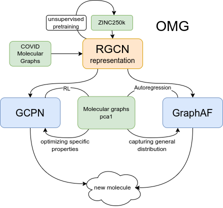
Graph Convolutional Policy Network (GCPN) and Graph Autoregressive Flow (GraphAF), RGCN is used as a base model for feature extraction. Before generating a new graph, both models need to understand the input graph’s features, such as node types and edge types, as well as any patterns or structures in the graph. After this, both models learn the “rules” of graph structure from their training data and then apply these rules when generating new graphs by different technique.
GCPN uses a reinforcement learning (RL) paradigm to fabricate molecules with refined chemical properties. This method aims to create molecules with particular properties by setting specific goals. The central strategy uses Graph Convolutional Policy Network (GCPN) and Proximal Policy Optimization (PPO).
Graph Convolutional Policy Network (GCPN): In the framework of molecular data, the GCPN, a deep learning model developed for graph structures, is found particularly fitting. Molecules are naturally represented as graphs, with atoms and bonds serving as nodes and edges, respectively. GCPN, a graph-based generative model, applies policy gradient methods for molecule generation. The generation process is sequential, selecting new atoms for addition and determining their connections to the existing molecule.
Proximal Policy Optimization (PPO): The PPO, a policy optimization method in reinforcement learning, aims at enhancing the policy while ensuring minimal deviation from the preceding policy. This approach aids in maintaining stability and securing reliable learning progress.
Fine-tuning with RL: The GCPN model, once pretrained, undergoes fine-tuning using reinforcement learning. The RL model sharpens its policy for generating molecules under the guidance of a reward function that assesses the chemical properties of the molecules. The generation of molecules with improved properties, such as enhanced drug-likeness, solubility, or synthetic accessibility, is the chief objective.
In the pretraining phase, a model is trained on a large dataset. The purpose of this step is to learn general features and patterns from the data. Here, the Relational Graph Convolutional Network (RGCN) model is trained on the ZINC250k dataset. The model is trained for 500 epochs with a batch size of 96. After the pretraining phase, the model is saved for later use.
import torch
from CovidMolGraph_TD import CovidMolGraphTD_imbalance
from torchdrug import datasets, data, utils, core, models, tasks
from torch import nn, optim

torch.manual_seed(42)

dataset_zinc250k = datasets.ZINC250k("./data/molecule-datasets/", kekulize=True, atom_feature="symbol")

model = models.RGCN(input_dim=dataset_zinc250k.node_feature_dim,
                    num_relation=dataset_zinc250k.num_bond_type,
                    hidden_dims=[256, 256, 256, 256], batch_norm=False)

task = tasks.GCPNGeneration(model, dataset_zinc250k.atom_types, max_edge_unroll=12,
                            max_node=38, criterion="nll")

optimizer = optim.Adam(task.parameters(), lr = 1e-3)

solver = core.Engine(task, dataset_zinc250k, None, None, optimizer,
                     gpus=[0, 1, 2, 3, 4, 5], batch_size=96, log_interval=100)

solver.train(num_epoch=500)
solver.save("./data/gcpn_dataset_zinc250k_500epoch.pkl")

dataset_covid = CovidMolGraphTD_imbalance("./data/CovidMolGraphTD_imbalance")

model = models.RGCN(input_dim=dataset_covid.node_feature_dim,
                    num_relation=dataset_covid.num_bond_type,
                    hidden_dims=[1024, 1024, 1024, 1024], batch_norm=True)

task = tasks.GCPNGeneration(model, dataset_covid.atom_types, max_edge_unroll=12,
                            max_node=38, criterion="nll")

optimizer = optim.Adam(task.parameters(), lr = 1e-3)

solver = core.Engine(task, dataset_covid, None, None, optimizer,
                     gpus=[0, 1, 2, 3, 4, 5], batch_size=128, log_interval=1000)

solver.train(num_epoch=1000)
solver.save("./data/gcpn_dataset_ncovid_1000epoch_batchnormalization_1024.pkl")
The next part of the experiment involves fine-tuning the pretrained model on a more specific task. This is where the model learns more task-specific patterns from a different dataset. In this case, the model is fine-tuned on a COVID-19 specific dataset using the Proximal Policy Optimization (PPO) algorithm, a reinforcement learning method. The learning rate is significantly lower than in the pretraining phase, indicating a more careful, incremental learning process. The model is trained for 100 epochs with a batch size of 16.
Loading the pretrained model for fine-tuning is performed with the optimizer state not being loaded. This implies that while the model parameters are loaded from the pretrained model, the state of the optimizer (which could include momentum, adaptive learning rates, etc.) is reinitialized.
Finally, the fine-tuned model is saved for further use or evaluation. The fine-tuned model is expected to perform better on the COVID-19 specific task than a model trained from scratch, thanks to the transfer of knowledge from the pretraining phase. This approach often reduces the amount of data required for the task-specific model and also shortens the training time.
import torch
from torchdrug import core, datasets, models, tasks
from torch import nn, optim
from collections import defaultdict

model = models.RGCN(input_dim=dataset_covid.node_feature_dim,
                    num_relation=dataset_covid.num_bond_type,
                    hidden_dims=[256, 256, 256, 256], batch_norm=True)
task = tasks.GCPNGeneration(model, dataset_covid.atom_types,
                            max_edge_unroll=12, max_node=38,
                            task=['pca1'], criterion="ppo",
                            reward_temperature=1,
                            agent_update_interval=3, gamma=0.9)


optimizer = optim.Adam(task.parameters(), lr=1e-5)
solver = core.Engine(task, dataset_covid, None, None, optimizer,
                     gpus=(0,), batch_size=16, log_interval=10)

solver.load("./data/gcpn_dataset_zinc250k_500epoch.pkl",load_optimizer=False)

# RL finetuning
solver.train(num_epoch=100)
solver.save("./data/gcpn_zinc250k_500epoch_finetune_covid_100epoch.pkl")
GraphAF, however, sequentially generates molecules atom by atom and bond by bond. This approach is rooted in the concept of normalizing flows in deep learning. It employs an invertible mapping between the types of nodes (atoms) and edges (bonds) in the molecular graph and a noise distribution. The main components of GraphAF include:
Relational Graph Convolutional Networks (RGCN): The RGCN serves as the graph representation model in GraphAF. It is a variant of GCN designed to handle graphs with varied relations or edges. In molecular terms, diverse types of edges can represent different chemical bonds.By utilizing an RGCN, GraphAF can learn a more expressive representation of the molecular graph that considers the types of bonds.
Autoregressive Generation: The training task for GraphAF, this process trains the model to generate the nodes and edges of the molecular graph sequentially. The generation process is autoregressive, implying that the generation of each new node or edge depends on the nodes and edges previously generated.
Node Flow Model and Edge Flow Model: These components, integral to the autoregressive generation task, define an invertible mapping between the types of nodes and edges in the molecular graph and noise distribution. By implementing a node flow model and an edge flow model, GraphAF can generate a diverse set of molecules.
2.3 Model Validation and Optimization
In the development of models, a strict validation, testing, and hyperparameter tuning procedure was employed, aimed at yielding reliable and robust performance.
The available dataset was partitioned into training, validation, and test subsets, thereby facilitating the impartial evaluation of the model. The training procedure of the model was intricately designed to generalize model performance to unseen data, the effectiveness of which was ascertained via this three-way dataset partitioning. Initial hyperparameters, including aspects like learning rate, weight decay, model embedding size, the number of attention heads, and dropout rate, among others, were pre-determined.
Throughout the training process, multiple epochs were executed. Upon the completion of each epoch, an evaluation of the model’s performance was carried out on the validation set. This evaluation involved the calculation of critical metrics, including balanced accuracy, recall, precision, and the F1-score for classification and R², MSE and RMSE for the regression task.
To prevent overfitting, a common pitfall in deep learning models, strategies like early stopping and model checkpointing, guided by validation metrics, were primarily utilized. Early stopping implies halting the training procedure once the model’s performance on the validation set no longer shows improvement. This method helps the model avoid becoming overly fitted to the training data, thus enhancing its ability to generalize.
Model checkpointing was adopted to preserve the model’s state when it demonstrated superior performance, as indicated by a higher average of recall, precision, and F1-score on the validation set compared to any previous epoch in classification and higher R² for regression. This method ensures that the model, which showed the highest generalization capacity during training, is retained for future predictive tasks.
The model was evaluated on the test set after finalizing the training and validation phase. This additional step was critical to provide a final confirmation of the model’s ability to generalize to completely unseen data. The model’s performance on the validation set also drove the refinement of hyperparameters. This approach to hyperparameter optimization allowed the model to be fine-tuned for the task at hand. These collective measures served to fortify the model’s ability to generalize and to inhibit overfitting, ensuring the model’s reliability and robustness.
2.4 Model Enhancement
Various strategies were employed to enhance the performance of the models used in this study. Two such approaches were the integration of models and the use of self-supervised learning.
In the discipline of machine learning, the fusion of distinct models is often employed, known as an ensemble approach, to optimize performance and accuracy. In the presented study, such an approach was adopted, integrating the BioGIP and GLMP models. Rather than using raw chemical feature vectors for node representation, latent embeddings sourced from the GLMP model were utilized. These embeddings, encompassing the molecules’ concentrated structural and physiochemical properties, were believed to provide a more in-depth and relevant portrayal of molecular properties. The anticipation was that this approach could improve the BioGIP model’s ability to classify or regress biological entities accurately.
Additionally, self-supervised learning was another key strategy used for model enhancement. In this method, models generate their labels from the input data, which has shown its effectiveness in predicting drug properties and molecule generation. Graph contrastive learning techniques such as InfoGraph[36] and Attribute Masking[37], which operate on graph-structured data and maximize the mutual information between node-level and graph-level representations, were used to enhance the GLMP model. Once trained, these models can generate meaningful representations of new graphs or nodes, useful in tasks like node classification, link prediction, or graph classification. This method was employed in the GLMP model to improve its ability to predict molecular properties.
In the generative model, OMG, self-supervised learning was incorporated in training the Relational Graph Convolutional Network (RGCN) model on the ZINC250k dataset. Therefore, this technique played a critical role in improving the accuracy of molecular property prediction (GLMP) and refining the molecule generation process (OMG). In the context of the OMG model, the role of the teacher model was essential in guiding the molecule generation process. The GCPN variant of the OMG model used a reinforcement learning (RL) framework, which characterized and evaluated the generated molecules based on their PCA1 value, a crucial descriptor of molecular properties as our primary objective. This evaluation was performed using an ordinal regressor model, thus enabling a more goal-oriented generation of molecules. The model, therefore, aimed to create molecules that optimize the targeted PCA1 value.
This study modified the OMG model’s source code to accommodate a custom task – the prediction of the PCA1 value. The novelty in this approach was the use of an ordinal regression instead of regression due to the poor performance of the latter. Hence, improvements to the predictor component of the OMG directly influenced the model’s effectiveness. The present study does not purport to pioneer new algorithms or models for graph generation. Rather, it focuses on the astute adaptation and implementation of well-known algorithms tailored explicitly for generating particular molecules. The study’s primary contribution is underscored by the intricate modifications enacted on existing models, ensuring their effective adaptation to bespoke tasks within the confines of this research.
2.5 Data acquisition, software and libraries
The Pharmaceutical Bioinformatics Research Group at Uppsala University provided cell profiling data for this study, which then preprocessed and normalized using the Python packages Polars and Pandas. The primary analysis, graph representation learning, was executed using Python, with the deep learning framework PyTorch and PyTorch Geometric and Deep Graph Library for graph neural networks implementation. Preprocessing and featurization of chemical compounds were done using DeepChem, with the RDKit and Mordred libraries used for physicochemical featurization. The TorchDrug toolkit was utilized to create network architectures for drug generation tasks.
Chemoinformatics operations were performed with RDKit, while Scikit-learn was used for machine learning tasks. Results were visualized using Plotly, and statistical analyses were performed in Python and R. This integrated approach revealed new interactions between chemical compounds, cellular phenotypes, and biological entities, identifying new potential drug targets.
This study capitalized on the computational prowess of Berzelius, an AI/ML focused compute cluster in Sweden using NVIDIA A100 GPUs, and in-house NVIDIA GTX 3090, hosted at Uppsala University’s Pharmaceutical Bioinformatics Research Group.
| Tool/Package | Description | Version | Additional Info |
|---|---|---|---|
| Python | Programming language | 3.8.10 | - |
| Polars | Data manipulation | 0.17.13 | - |
| Pandas | Data manipulation | 1.5.3 | - |
| PyTorch | Deep learning framework | 1.13.1+cu116 | - |
| PyTorch Geometric | Graph representation learning | 2.2.0 | Extension of PyTorch |
| Deep Graph Library (DGL) | Graph representation learning | 1.0.1+cu116 | Extension of PyTorch |
| DeepChem | Chemoinformatics | 2.7.1 | Used for pre-processing and featurization |
| RDKit | Chemoinformatics | 2022.09.5 | Used for physico-chemical featurization |
| Mordred | Chemoinformatics | Latest | Used for physico-chemical featurization |
| TorchDrug | Drug discovery toolkit | 0.2.0.post1 | Used for network architectures |
| Scikit-learn | Machine Learning | 1.2.1 | Used for model evaluation and comparing models |
| BioTransformers | ESM/Protbert models | 0.1.17 | Protein featurization |
| Plotly | Data visualization | 5.14.1 | - |
| R | Statistical analysis | 4.2.2 | Used for specific statistical analyses |