3 Result and Discussion
3.1 Regression/Classification Performance
The performance of multiple machine learning models, such as the GLMP and BioGIP, was assessed through various tasks. Detailed results can be found in Appendix A.
A variety of conventional models such as Gradient Boosting (GBoost), Random Forest (RF), K-Nearest Neighbors, Decision Tree, Multi-layer Perceptron (MLP), Support Vector Machines Classifier/Regressor (SVC/SVR), AdaBoost, Gaussian Naive Bayes/Gaussian Process, Stochastic Gradient Descent (SGD), and Ridge Regression were included for comparison. While these models exhibited marginally better performance than the conventional models, it was clear that improvements were needed in their ability to perform regression on the PCA1 value. Currently, these models are not optimally suitable for regression tasks (Comparative Performance of Models Table).
Comparative Performance of Models on PCA1 Classification and Regression Tasks: This table presents the best-observed performance of GLMP and BioGIP models, contrasted with several conventional models. For input, conventional models and GLMP use a feature vector encompassing structural and physicochemical properties of molecules. GLMP further integrates this with global graph presentations of molecules. BioGIP employs distinct node features (chemical, protein, and pathways) and their links. When GLMP and BioGIP are connected, the chemical feature becomes the last layer of the GLMP model.
| GLMP | BioGIP | GBoost | RF | KNNeighbors | DecisionTree | MLP | SVC/SVR | AdaBoost | Gaussian NB/Process | SGD | Ridge | |
|---|---|---|---|---|---|---|---|---|---|---|---|---|
| AUC-ROC | 0.63 | 0.75 | 0.57 | 0.5 | 0.52 | 0.58 | 0.57 | 0.56 | 0.5 | 0.62 | 0.6 | |
| Balanced Accuracy | 0.58 | 0.72 | 0.57 | 0.5 | 0.52 | 0.58 | 0.57 | 0.56 | 0.5 | 0.62 | 0.6 | |
| Recall | 0.26 | 0.75 | 0.19 | 0 | 0.04 | 0.19 | 0.15 | 0.15 | 0 | 0.37 | 0.22 | |
| Precision | 0.54 | 0.58 | 0.11 | 0 | 0.17 | 0.17 | 0.25 | 0.18 | 0 | 0.07 | 0.19 | |
| F1 | 0.36 | 0.60 | 0.14 | 0 | 0.06 | 0.18 | 0.19 | 0.16 | 0 | 0.12 | 0.2 | |
| \(R^2\) | 0.16 | 0.07 | 0 | 0.03 | 0.04 | 0 | $<$0 | 0.05 | 0.03 | $<$0 | $<$0 | |
| mse | 4.89 | 5.25 | 5.56 | 5.36 | 5.31 | 5.54 | 6.24 | 5.27 | 5.38 | 6.36 | 7.49 | |
| rmse | 2.21 | 2.29 | 2.36 | 2.32 | 2.31 | 2.35 | 2.5 | 2.3 | 2.32 | 2.52 | 2.74 |
In the classification tasks, an interesting pattern was observed. The BioGIP model demonstrated superior performance across most metrics, including AUC-ROC, Balanced Accuracy, Recall, Precision, and F1-Score. However, when it came to the regression tasks, the GLMP and an enhanced version of GLMP, GLMP-PreGIN, displayed a higher R\(^2\) value and lower mean squared error (MSE) and root mean squared error (RMSE), potentially suggesting a better fit of the model to the data.
Further experiment was conducted by introducing different GLMP and BioGIP model enhancement approaches. Here, the GLMP-BioGIP model yielded the best performance across both classification and regression tasks, as indicated by the metrics (Performance of Enhanced Models on Classification and Regression Table).
Performance of Enhanced Models on Classification and Regression Tasks: This table compares the performance of different model enhancement approaches on GLMP and BioGIP models.
| GLMP | GLMP-PreGIN | BioGIP\(_{\text{seq}}\) | BioGIP\(_{\text{cat}}\) | BioGIP\(_{\text{res}}\) | GLMP-BioGIP | |
|---|---|---|---|---|---|---|
| AUC-ROC | 0.61 | 0.63 | 0.75 | 0.69 | 0.59 | 0.78 |
| Balanced Accuracy | 0.56 | 0.58 | 0.72 | 0.68 | 0.55 | 0.71 |
| Recall | 0.21 | 0.26 | 0.75 | 0.62 | 0.53 | 0.77 |
| Precision | 0.18 | 0.54 | 0.58 | 0.53 | 0.51 | 0.62 |
| F1 | 0.2 | 0.36 | 0.6 | 0.51 | 0.44 | 0.66 |
| \(R^2\) | 0.01 | 0.16 | 0.07 | 0.03 | 0 | 0.17 |
| mse | 5.49 | 4.89 | 5.26 | 5.35 | 5.6 | 4.87 |
| rmse | 2.34 | 2.21 | 2.29 | 2.31 | 2.37 | 2.20 |
3.2 COVID-19 BioGraph Topology
The COVID-19 BioGraph is a comprehensive network of several key components - chemicals, proteins, and biological pathways. These elements are intricately interconnected, forming a complex topology that underscores the dynamism of biological systems.
Of the 4,293 chemicals represented in the BioGraph, 3,711 are known to interact with at least one protein. This highlights chemicals’ crucial role in influencing protein function, indicating a high degree of interaction between these two entities.
The total number of proteins in the BioGraph is 16,733, with a striking 16,727 shown to interact with chemicals. The near-universal interaction between proteins and chemicals reinforces their integral role in maintaining and regulating biological processes.
The BioGraph also features 1,117 unique biological pathways. However, only 282 proteins are identified as governing these pathways, demonstrating a subset of proteins’ pivotal role in controlling and influencing various biological processes. The role of chemicals is again emphasized as it is found that 3,220 of them are linked to all biological pathways. This widespread involvement of chemicals in biological pathways indicates their significant influence on the overall functioning of biological processes.
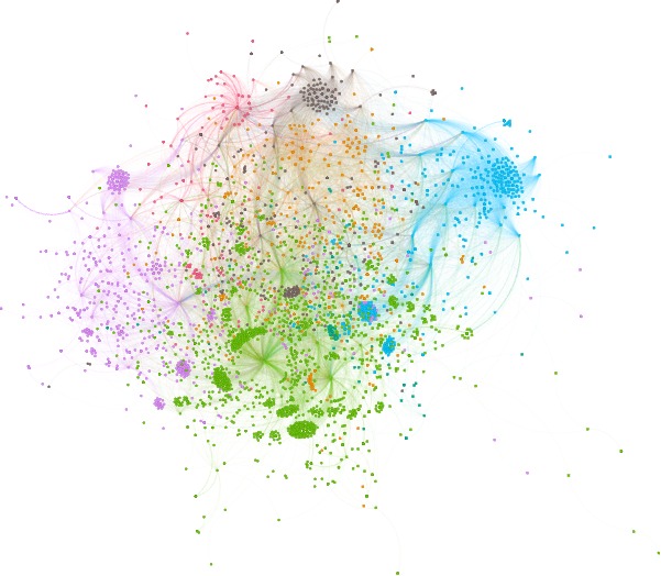
A subgraph of the BioGraph, focusing on 136 active compounds, has been depicted for a more manageable analysis. There are three different types of nodes in this subgraph - green, pink, and blue - representing compounds, pathways, and proteins. The size of the green nodes represents the degree of the compounds, thus offering a visual representation of their connectivity within the network.
In the active subgraph, module detection has been employed to identify interconnected communities of compounds related to specific proteins and pathways. This method potentially reveals disparate mechanisms by highlighting unique compound-protein-pathway interactions.
3.3 Combination Prediction
Finding active chemical combinations within inactive compounds was obtained by implementing two distinct strategies aimed at predicting the joint effect of nodes, or chemical combinations, in the BioGraph. The methods used were the PCA1 range selection and the louvain community detection algorithm, both of which facilitated the selection of hypothetical inactive nodes that could potentially make an active combination.
In the first approach, an emphasis was placed on employing PCA1 values, specifically those ranging between 2.9 and 5, in selecting chemical compounds for combination. This particular range was chosen due to its proximity to the values exhibited by active compounds. The technique led to the selection of 141 nodes (molecules), thereby reducing the computational burden by limiting the potential compound combinations to a manageable 9,871 pairs.
In the second strategy, the louvain community detection algorithm was utilized to select promising inactive nodes. With its capability of revealing hidden patterns and reducing network complexity, this algorithm proved to be a potent alternative to PCA1-based compound selection. It yielded 159 compounds for combination and a total of 12,561 possible combinations.
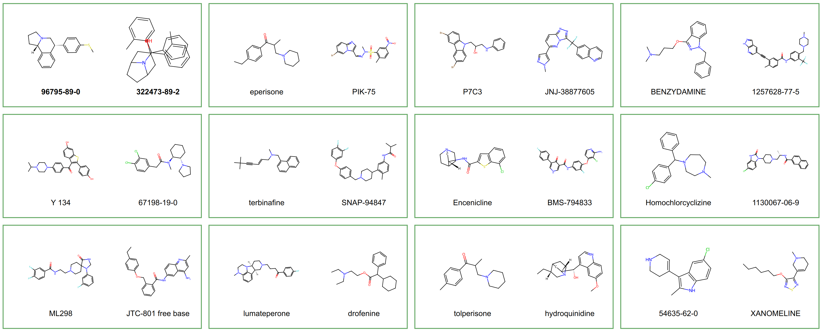
The selected combinations were then tested using our most effective model, BioGIP-GLMP. As a result, 1519 combinations from the first approach (representing 15.4% of the total) and 1183 combinations from the second approach (amounting to 9.4% of the total) were identified as active, with a probability range of 0.5 to 1.
A number of these combinations are shown in the figure above. Notably, there was a significant overlap between the results of both strategies. Of the identified active combinations, 298 pairs were similar in both approaches, representing approximately 20% of the active combinations from the PCA1 range selection method and 25% from the louvain community detection approach.
A vital caveat to note in the PCA1 approach is that the number of inactive compounds within the selected range remained fixed. However, for the louvain community detection method, the number of identified communities and the population of active compounds within these communities varied depending on the chosen resolution. Furthermore, as the louvain community detection algorithm uses a random approach to identify modularity, the results differed with each iteration.
At resolution 1, between 11 to 16 distinct modules were typically identified, with active compounds scattered across half of them. A growing separation between active and inactive compounds within the communities was observed as the resolution was incrementally increased. Nevertheless, several mixed communities persisted. These mixed communities, containing both active and inactive compounds, offered intriguing possibilities as they contained inactive compounds that could potentially behave like active compounds within the class. Consequently, they were considered good candidates for combination.
Finally, an adjustment was set to level 7, with all communities possessing at least 20% active compound. These communities were consequently isolated. Subsequently, the inactive compounds for combination were segregated within these isolated communities.
3.4 Molecule Generation
As part of the OMG model, a suite of graph-based generative models was employed to generate optimized molecules, namely, the Graph Convolutional Policy Network (GCPN) and GraphAF. These models were founded on the premise of understanding the input graph’s inherent features, such as node types and edge types, which facilitated the generation of new graphs. The performance of these models was then evaluated using an ordinal regression model, an alternative to the less successful GLMP and BioGIP regressor models, which showed poor regression performance with an R\(^2\) of 0.17 at their best.
The ordinal regression model was utilized because of its ability to overcome the inadequacies of the other models. It simplifies the problem of quantifying the goodness of a generated molecule, making it a suitable measure for the reinforcement learning paradigm used by OMG. The model segmented the PCA1 value into ordinal categories, facilitating a more straightforward interpretation of the order of goodness of the generated molecules.
The PCA1 value was divided into five categories as per the ordinal regression: (-12, -5), (-5, 2), (2, 9), (9, 16). The results showed that the model performed relatively well, with an overall accuracy of 56.36%. It was noted that the model performed best on molecules with PCA1 values within class 2 (-5, 2), yielding the highest f1-score. On closer inspection of the results, it was found that the compounds with PCA1 values above five were often classified within class 3 (2, 9), with a lesser number falling within class 4 (9, 16). However, a decision was made to count molecules with PCA1 values above nine active, not those above five, to ensure a stringent definition of an “active” compound during the training phase. This choice made the model more conservative, thus reducing the risk of generating false positives.
Regarding the specific attributes of the generated molecules, both GCPN and GraphAF offered unique benefits. Molecules generated by GraphAF were generally simpler and smaller, often incorporating atoms other than carbon, which could potentially lead to better solubility and decreased hydrophobicity. Conversely, GCPN tended to generate more complex molecules, indicating these models’ versatility in producing various molecular structures.
Overall, the ordinal regression model proved beneficial for evaluating the molecules generated by the OMG models. By adopting a conservative stance during training, the model mitigated the risk of producing false positives, thus offering potential avenues for future research in optimized molecular generation.